devtools::install_github("lukeCe/spflow")Skipping install of 'spflow' from a github remote, the SHA1 (df913677) has not changed since last install.
Use `force = TRUE` to force installationdevtools::install_github("lukeCe/spflow")Skipping install of 'spflow' from a github remote, the SHA1 (df913677) has not changed since last install.
Use `force = TRUE` to force installationpacman::p_load(tmap, sf, spdep, sp, Matrix,
spflow, reshape2, knitr,
tidyverse)mpsz <- st_read(dsn = "data/geospatial",
layer = "MPSZ-2019") %>%
st_transform(crs = 3414) Reading layer `MPSZ-2019' from data source
`/Users/linxu/ISSS624/in-class exercise 5/data/geospatial'
using driver `ESRI Shapefile'
Simple feature collection with 332 features and 6 fields
Geometry type: MULTIPOLYGON
Dimension: XY
Bounding box: xmin: 103.6057 ymin: 1.158699 xmax: 104.0885 ymax: 1.470775
Geodetic CRS: WGS 84busstop <- st_read(dsn = "data/geospatial",
layer = "BusStop") %>%
st_transform(crs = 3414)Reading layer `BusStop' from data source
`/Users/linxu/ISSS624/in-class exercise 5/data/geospatial'
using driver `ESRI Shapefile'
Simple feature collection with 5159 features and 3 fields
Geometry type: POINT
Dimension: XY
Bounding box: xmin: 3970.122 ymin: 26482.1 xmax: 48280.78 ymax: 52983.82
Projected CRS: SVY21mpsz$`BUSSTOP_COUNT`<- lengths(
st_intersects(
mpsz, busstop))mpsz_busstop <- mpsz %>%
filter(BUSSTOP_COUNT > 0)
mpsz_busstopSimple feature collection with 313 features and 7 fields
Geometry type: MULTIPOLYGON
Dimension: XY
Bounding box: xmin: 2667.538 ymin: 21448.47 xmax: 50271.73 ymax: 50256.33
Projected CRS: SVY21 / Singapore TM
First 10 features:
SUBZONE_N SUBZONE_C PLN_AREA_N PLN_AREA_C REGION_N
1 INSTITUTION HILL RVSZ05 RIVER VALLEY RV CENTRAL REGION
2 ROBERTSON QUAY SRSZ01 SINGAPORE RIVER SR CENTRAL REGION
3 FORT CANNING MUSZ02 MUSEUM MU CENTRAL REGION
4 MARINA EAST (MP) MPSZ05 MARINE PARADE MP CENTRAL REGION
5 SENTOSA SISZ01 SOUTHERN ISLANDS SI CENTRAL REGION
6 CITY TERMINALS BMSZ17 BUKIT MERAH BM CENTRAL REGION
7 ANSON DTSZ10 DOWNTOWN CORE DT CENTRAL REGION
8 STRAITS VIEW SVSZ01 STRAITS VIEW SV CENTRAL REGION
9 MARITIME SQUARE BMSZ01 BUKIT MERAH BM CENTRAL REGION
10 TELOK BLANGAH RISE BMSZ15 BUKIT MERAH BM CENTRAL REGION
REGION_C geometry BUSSTOP_COUNT
1 CR MULTIPOLYGON (((28481.45 30... 2
2 CR MULTIPOLYGON (((28087.34 30... 10
3 CR MULTIPOLYGON (((29542.53 31... 6
4 CR MULTIPOLYGON (((35279.55 30... 2
5 CR MULTIPOLYGON (((26879.04 26... 1
6 CR MULTIPOLYGON (((27891.15 28... 10
7 CR MULTIPOLYGON (((29201.07 28... 5
8 CR MULTIPOLYGON (((31269.21 28... 4
9 CR MULTIPOLYGON (((26920.02 26... 21
10 CR MULTIPOLYGON (((27483.57 28... 11centroids <- suppressWarnings({
st_point_on_surface(st_geometry(mpsz_busstop))})
mpsz_nb <- list(
"by_contiguity" = poly2nb(mpsz_busstop),
"by_distance" = dnearneigh(centroids,
d1 = 0, d2 = 5000),
"by_knn" = knn2nb(knearneigh(centroids, 3))
)mpsz_nb$by_contiguity
Neighbour list object:
Number of regions: 313
Number of nonzero links: 1902
Percentage nonzero weights: 1.94143
Average number of links: 6.076677
$by_distance
Neighbour list object:
Number of regions: 313
Number of nonzero links: 15422
Percentage nonzero weights: 15.74171
Average number of links: 49.27157
1 region with no links:
313
2 disjoint connected subgraphs
$by_knn
Neighbour list object:
Number of regions: 313
Number of nonzero links: 939
Percentage nonzero weights: 0.9584665
Average number of links: 3
Non-symmetric neighbours listplot(st_geometry(mpsz))
plot(mpsz_nb$by_contiguity,
centroids,
add = T,
col = rgb(0,0,0,
alpha=0.5))
title("Contiguity") 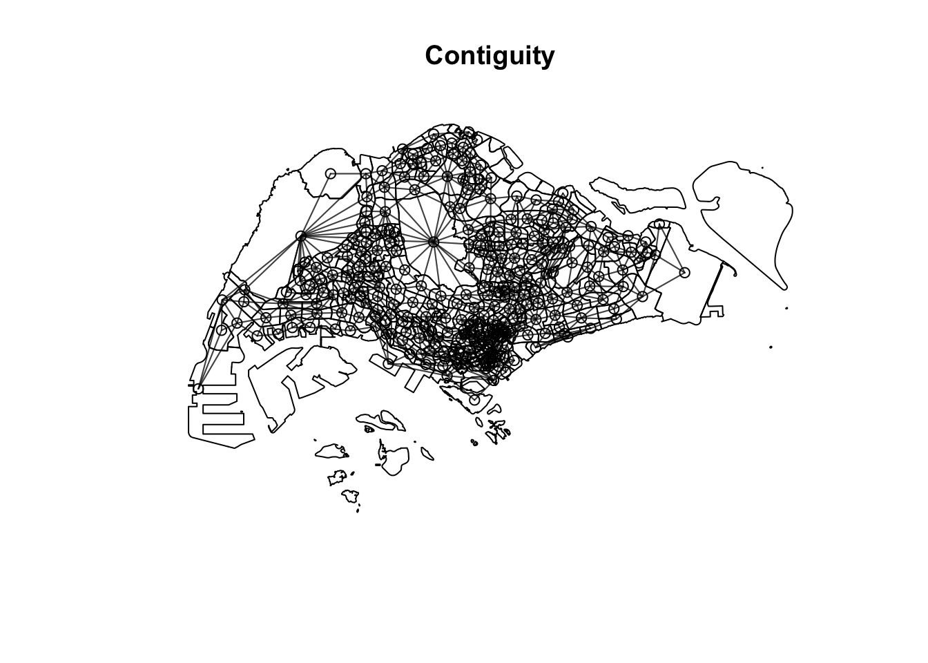
plot(st_geometry(mpsz))
plot(mpsz_nb$by_distance,
     centroids,
     add = T,
     col = rgb(0,0,0,
               alpha=0.5))
title("Distance") 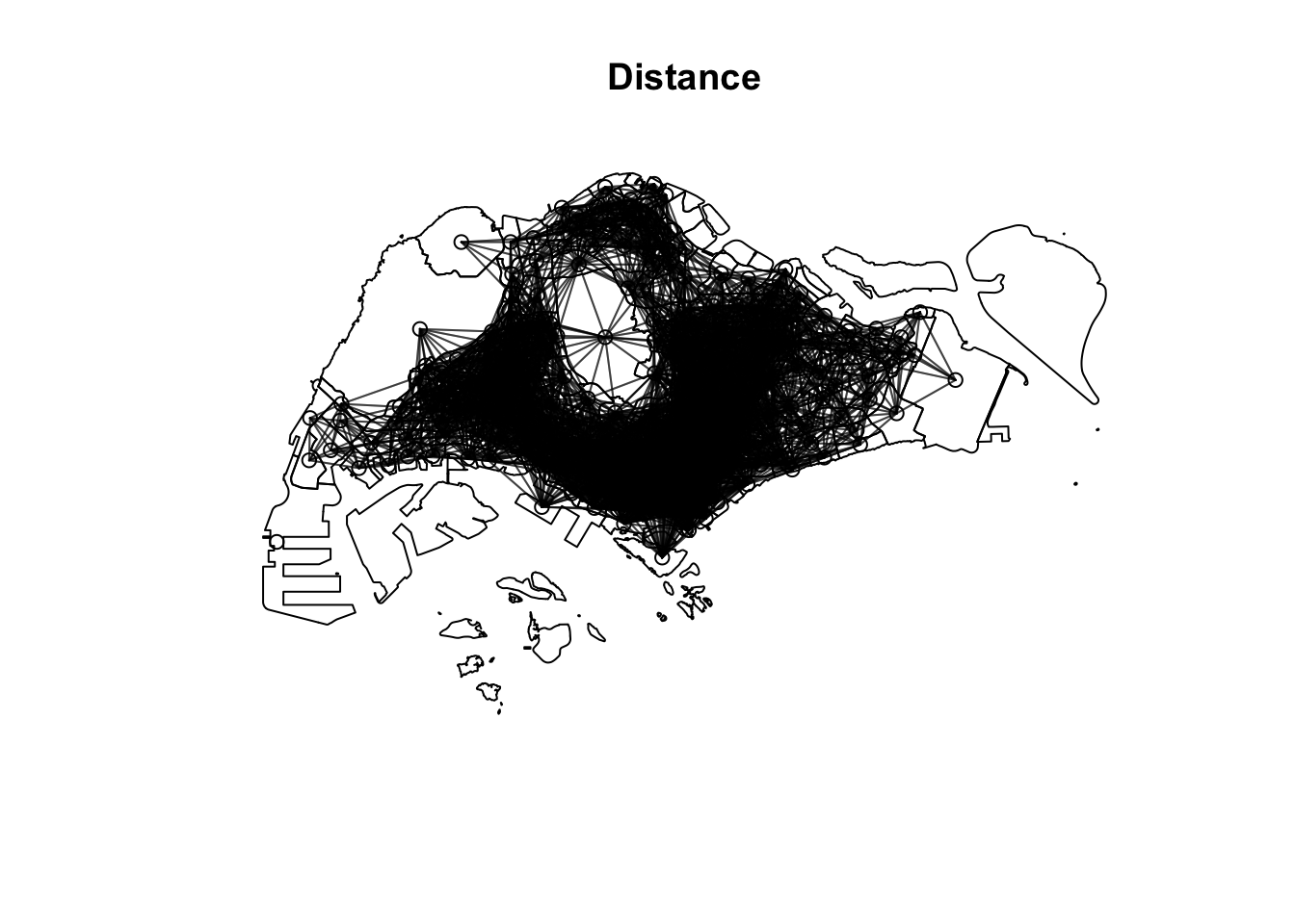
plot(st_geometry(mpsz))
plot(mpsz_nb$by_knn,
     centroids,
     add = T,
     col = rgb(0,0,0,
               alpha=0.5))
title("3 Nearest Neighbors") 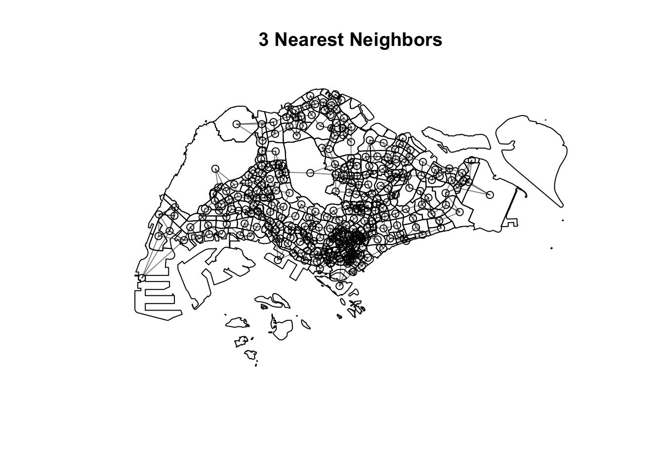
write_rds(mpsz_nb, "data/rds/mpsz_nb.rds")odbus6_9 <- read_rds("data/rds/odbus6_9.rds")busstop_mpsz <- st_intersection(busstop, mpsz) %>%
select(BUS_STOP_N, SUBZONE_C) %>%
st_drop_geometry()Warning: attribute variables are assumed to be spatially constant throughout
all geometriesod_data <- left_join(odbus6_9 , busstop_mpsz,
by = c("ORIGIN_PT_CODE" = "BUS_STOP_N")) %>%
rename(ORIGIN_BS = ORIGIN_PT_CODE,
ORIGIN_SZ = SUBZONE_C,
DESTIN_BS = DESTINATION_PT_CODE)Warning in left_join(odbus6_9, busstop_mpsz, by = c(ORIGIN_PT_CODE = "BUS_STOP_N")): Detected an unexpected many-to-many relationship between `x` and `y`.
ℹ Row 55491 of `x` matches multiple rows in `y`.
ℹ Row 161 of `y` matches multiple rows in `x`.
ℹ If a many-to-many relationship is expected, set `relationship =
"many-to-many"` to silence this warning.duplicate <- od_data %>%
group_by_all() %>%
filter(n()>1) %>%
ungroup()od_data <- unique(od_data)od_data <- left_join(od_data , busstop_mpsz,
by = c("DESTIN_BS" = "BUS_STOP_N")) Warning in left_join(od_data, busstop_mpsz, by = c(DESTIN_BS = "BUS_STOP_N")): Detected an unexpected many-to-many relationship between `x` and `y`.
ℹ Row 74 of `x` matches multiple rows in `y`.
ℹ Row 1379 of `y` matches multiple rows in `x`.
ℹ If a many-to-many relationship is expected, set `relationship =
"many-to-many"` to silence this warning.duplicate <- od_data %>%
group_by_all() %>%
filter(n()>1) %>%
ungroup()od_data <- unique(od_data)od_data <- od_data %>%
rename(DESTIN_SZ = SUBZONE_C) %>%
drop_na() %>%
group_by(ORIGIN_SZ, DESTIN_SZ) %>%
summarise(TRIPS = sum(TRIPS))`summarise()` has grouped output by 'ORIGIN_SZ'. You can override using the
`.groups` argument.kable(head(od_data, n = 5))| ORIGIN_SZ | DESTIN_SZ | TRIPS |
|---|---|---|
| AMSZ01 | AMSZ01 | 1998 |
| AMSZ01 | AMSZ02 | 8289 |
| AMSZ01 | AMSZ03 | 8971 |
| AMSZ01 | AMSZ04 | 2252 |
| AMSZ01 | AMSZ05 | 6136 |
write_rds(od_data, "data/rds/od_data.rds")mpsz_sp <- as(mpsz_busstop, "Spatial")
mpsz_spclass : SpatialPolygonsDataFrame
features : 313
extent : 2667.538, 50271.73, 21448.47, 50256.33 (xmin, xmax, ymin, ymax)
crs : +proj=tmerc +lat_0=1.36666666666667 +lon_0=103.833333333333 +k=1 +x_0=28001.642 +y_0=38744.572 +ellps=WGS84 +towgs84=0,0,0,0,0,0,0 +units=m +no_defs
variables : 7
names : SUBZONE_N, SUBZONE_C, PLN_AREA_N, PLN_AREA_C, REGION_N, REGION_C, BUSSTOP_COUNT
min values : ADMIRALTY, AMSZ01, ANG MO KIO, AM, CENTRAL REGION, CR, 1
max values : YUNNAN, YSSZ09, YISHUN, YS, WEST REGION, WR, 87 DISTANCE <- spDists(mpsz_sp,
longlat = FALSE)head(DISTANCE, n=c(10, 10)) [,1] [,2] [,3] [,4] [,5] [,6] [,7] [,8]
[1,] 0.0000 305.737 951.8314 5254.066 4975.002 3176.159 2345.174 3455.579
[2,] 305.7370 0.000 1045.9088 5299.849 4669.295 2873.497 2074.691 3277.921
[3,] 951.8314 1045.909 0.0000 4303.232 5226.873 3341.212 2264.201 2890.870
[4,] 5254.0664 5299.849 4303.2323 0.000 7707.091 6103.071 5007.197 3699.242
[5,] 4975.0021 4669.295 5226.8731 7707.091 0.000 1893.049 3068.627 4009.437
[6,] 3176.1592 2873.497 3341.2116 6103.071 1893.049 0.000 1200.264 2532.383
[7,] 2345.1741 2074.691 2264.2014 5007.197 3068.627 1200.264 0.000 1709.443
[8,] 3455.5791 3277.921 2890.8696 3699.242 4009.437 2532.383 1709.443 0.000
[9,] 3860.6063 3612.345 4570.3316 8324.615 2766.650 2606.583 3383.338 5032.870
[10,] 2634.7332 2358.403 3255.0325 6981.431 2752.882 1666.022 2115.640 3815.333
[,9] [,10]
[1,] 3860.606 2634.733
[2,] 3612.345 2358.403
[3,] 4570.332 3255.033
[4,] 8324.615 6981.431
[5,] 2766.650 2752.882
[6,] 2606.583 1666.022
[7,] 3383.338 2115.640
[8,] 5032.870 3815.333
[9,] 0.000 1357.426
[10,] 1357.426 0.000sz_names <- mpsz_busstop$SUBZONE_Ccolnames(DISTANCE) <- paste0(sz_names)
rownames(DISTANCE) <- paste0(sz_names)distPair <- melt(DISTANCE) %>%
rename(DISTANCE = value)
head(distPair, 10) Var1 Var2 DISTANCE
1 RVSZ05 RVSZ05 0.0000
2 SRSZ01 RVSZ05 305.7370
3 MUSZ02 RVSZ05 951.8314
4 MPSZ05 RVSZ05 5254.0664
5 SISZ01 RVSZ05 4975.0021
6 BMSZ17 RVSZ05 3176.1592
7 DTSZ10 RVSZ05 2345.1741
8 SVSZ01 RVSZ05 3455.5791
9 BMSZ01 RVSZ05 3860.6063
10 BMSZ15 RVSZ05 2634.7332distPair <- distPair %>%
rename(ORIGIN_SZ = Var1,
DESTIN_SZ = Var2)flow_data <- distPair %>%
left_join (od_data) %>%
mutate(TRIPS = coalesce(TRIPS, 0))Joining with `by = join_by(ORIGIN_SZ, DESTIN_SZ)`kable(head(flow_data, n = 10))| ORIGIN_SZ | DESTIN_SZ | DISTANCE | TRIPS |
|---|---|---|---|
| RVSZ05 | RVSZ05 | 0.0000 | 67 |
| SRSZ01 | RVSZ05 | 305.7370 | 549 |
| MUSZ02 | RVSZ05 | 951.8314 | 0 |
| MPSZ05 | RVSZ05 | 5254.0664 | 0 |
| SISZ01 | RVSZ05 | 4975.0021 | 0 |
| BMSZ17 | RVSZ05 | 3176.1592 | 0 |
| DTSZ10 | RVSZ05 | 2345.1741 | 0 |
| SVSZ01 | RVSZ05 | 3455.5791 | 0 |
| BMSZ01 | RVSZ05 | 3860.6063 | 0 |
| BMSZ15 | RVSZ05 | 2634.7332 | 0 |
write_rds(flow_data, "data/rds/mpsz_flow.rds")pop <- read_csv("data/aspatial/pop.csv")Rows: 332 Columns: 5
── Column specification ────────────────────────────────────────────────────────
Delimiter: ","
chr (2): PA, SZ
dbl (3): AGE7_12, AGE13_24, AGE25_64
ℹ Use `spec()` to retrieve the full column specification for this data.
ℹ Specify the column types or set `show_col_types = FALSE` to quiet this message.mpsz_var <- mpsz_busstop %>%
left_join(pop,
by = c("PLN_AREA_N" = "PA",
"SUBZONE_N" = "SZ")) %>%
select(1:2, 7:11) %>%
rename(SZ_NAME = SUBZONE_N,
SZ_CODE = SUBZONE_C)kable(head(mpsz_var[, 1:6], n = 6))| SZ_NAME | SZ_CODE | BUSSTOP_COUNT | AGE7_12 | AGE13_24 | AGE25_64 | geometry |
|---|---|---|---|---|---|---|
| INSTITUTION HILL | RVSZ05 | 2 | 330 | 360 | 2260 | MULTIPOLYGON (((28481.45 30… |
| ROBERTSON QUAY | SRSZ01 | 10 | 320 | 350 | 2200 | MULTIPOLYGON (((28087.34 30… |
| FORT CANNING | MUSZ02 | 6 | 0 | 10 | 30 | MULTIPOLYGON (((29542.53 31… |
| MARINA EAST (MP) | MPSZ05 | 2 | 0 | 0 | 0 | MULTIPOLYGON (((35279.55 30… |
| SENTOSA | SISZ01 | 1 | 200 | 260 | 1440 | MULTIPOLYGON (((26879.04 26… |
| CITY TERMINALS | BMSZ17 | 10 | 0 | 0 | 0 | MULTIPOLYGON (((27891.15 28… |
schools <- read_rds("data/rds/schools.rds")mpsz_var$`SCHOOL_COUNT`<- lengths(
st_intersects(
mpsz_var, schools))business <- st_read(dsn = "data/geospatial",
layer = "Business") %>%
st_transform(crs = 3414)Reading layer `Business' from data source
`/Users/linxu/ISSS624/in-class exercise 5/data/geospatial'
using driver `ESRI Shapefile'
Simple feature collection with 6550 features and 3 fields
Geometry type: POINT
Dimension: XY
Bounding box: xmin: 3669.148 ymin: 25408.41 xmax: 47034.83 ymax: 50148.54
Projected CRS: SVY21 / Singapore TMretails <- st_read(dsn = "data/geospatial",
layer = "Retails") %>%
st_transform(crs = 3414)Reading layer `Retails' from data source
`/Users/linxu/ISSS624/in-class exercise 5/data/geospatial'
using driver `ESRI Shapefile'
Simple feature collection with 37635 features and 3 fields
Geometry type: POINT
Dimension: XY
Bounding box: xmin: 4737.982 ymin: 25171.88 xmax: 48265.04 ymax: 50135.28
Projected CRS: SVY21 / Singapore TMfinserv <- st_read(dsn = "data/geospatial",
layer = "FinServ") %>%
st_transform(crs = 3414)Reading layer `FinServ' from data source
`/Users/linxu/ISSS624/in-class exercise 5/data/geospatial'
using driver `ESRI Shapefile'
Simple feature collection with 3320 features and 3 fields
Geometry type: POINT
Dimension: XY
Bounding box: xmin: 4881.527 ymin: 25171.88 xmax: 46526.16 ymax: 49338.02
Projected CRS: SVY21 / Singapore TMentertn <- st_read(dsn = "data/geospatial",
layer = "entertn") %>%
st_transform(crs = 3414)Reading layer `entertn' from data source
`/Users/linxu/ISSS624/in-class exercise 5/data/geospatial'
using driver `ESRI Shapefile'
Simple feature collection with 114 features and 3 fields
Geometry type: POINT
Dimension: XY
Bounding box: xmin: 10809.34 ymin: 26528.63 xmax: 41600.62 ymax: 46375.77
Projected CRS: SVY21 / Singapore TMfb <- st_read(dsn = "data/geospatial",
layer = "F&B") %>%
st_transform(crs = 3414)Reading layer `F&B' from data source
`/Users/linxu/ISSS624/in-class exercise 5/data/geospatial'
using driver `ESRI Shapefile'
Simple feature collection with 1919 features and 3 fields
Geometry type: POINT
Dimension: XY
Bounding box: xmin: 6010.495 ymin: 25343.27 xmax: 45462.43 ymax: 48796.21
Projected CRS: SVY21 / Singapore TMlr <- st_read(dsn = "data/geospatial",
layer = "Liesure&Recreation") %>%
st_transform(crs = 3414)Reading layer `Liesure&Recreation' from data source
`/Users/linxu/ISSS624/in-class exercise 5/data/geospatial'
using driver `ESRI Shapefile'
Simple feature collection with 1217 features and 30 fields
Geometry type: POINT
Dimension: XY
Bounding box: xmin: 6010.495 ymin: 25134.28 xmax: 48439.77 ymax: 50078.88
Projected CRS: SVY21 / Singapore TMmpsz_var$`BUSINESS_COUNT`<- lengths(
st_intersects(
mpsz_var, business))
mpsz_var$`RETAILS_COUNT`<- lengths(
st_intersects(
mpsz_var, retails))
mpsz_var$`FINSERV_COUNT`<- lengths(
st_intersects(
mpsz_var, finserv))
mpsz_var$`ENTERTN_COUNT`<- lengths(
st_intersects(
mpsz_var, entertn))
mpsz_var$`FB_COUNT`<- lengths(
st_intersects(
mpsz_var, fb))
mpsz_var$`LR_COUNT`<- lengths(
st_intersects(
mpsz_var, lr))glimpse(mpsz_var)Rows: 313
Columns: 14
$ SZ_NAME <chr> "INSTITUTION HILL", "ROBERTSON QUAY", "FORT CANNING", "…
$ SZ_CODE <chr> "RVSZ05", "SRSZ01", "MUSZ02", "MPSZ05", "SISZ01", "BMSZ…
$ BUSSTOP_COUNT <int> 2, 10, 6, 2, 1, 10, 5, 4, 21, 11, 2, 9, 6, 1, 4, 7, 24,…
$ AGE7_12 <dbl> 330, 320, 0, 0, 200, 0, 0, 0, 350, 470, 0, 300, 390, 0,…
$ AGE13_24 <dbl> 360, 350, 10, 0, 260, 0, 0, 0, 460, 1160, 0, 760, 890, …
$ AGE25_64 <dbl> 2260, 2200, 30, 0, 1440, 0, 0, 0, 2600, 6260, 630, 4350…
$ geometry <MULTIPOLYGON [m]> MULTIPOLYGON (((28481.45 30..., MULTIPOLYG…
$ SCHOOL_COUNT <int> 1, 0, 0, 0, 0, 0, 0, 0, 0, 2, 0, 1, 1, 0, 0, 0, 1, 0, 0…
$ BUSINESS_COUNT <int> 6, 4, 7, 0, 1, 11, 15, 1, 10, 1, 17, 6, 0, 0, 51, 2, 3,…
$ RETAILS_COUNT <int> 26, 207, 17, 0, 84, 14, 52, 0, 460, 34, 263, 55, 37, 1,…
$ FINSERV_COUNT <int> 3, 18, 0, 0, 29, 4, 6, 0, 34, 4, 26, 4, 3, 6, 59, 3, 8,…
$ ENTERTN_COUNT <int> 0, 6, 3, 0, 2, 0, 0, 0, 1, 0, 0, 0, 0, 0, 3, 0, 0, 0, 0…
$ FB_COUNT <int> 4, 38, 4, 0, 38, 15, 5, 0, 20, 0, 9, 25, 0, 0, 9, 1, 3,…
$ LR_COUNT <int> 3, 11, 7, 0, 20, 0, 0, 0, 19, 2, 4, 4, 1, 1, 13, 0, 17,…write_rds(mpsz_var, "data/rds/mpsz_var.rds")mpsz_nb <- read_rds("data/rds/mpsz_nb.rds")
mpsz_flow <- read_rds("data/rds/mpsz_flow.rds")
mpsz_var <- read_rds("data/rds/mpsz_var.rds")mpsz_net <- spflow_network(
id_net = "sg",
node_neighborhood = nb2mat(mpsz_nb$by_contiguity),
node_data = mpsz_var,
node_key_column = "SZ_CODE")
mpsz_netSpatial network nodes with id: sg
--------------------------------------------------
Number of nodes: 313
Average number of links per node: 6.077
Density of the neighborhood matrix: 1.94% (non-zero connections)
Data on nodes:
SZ_NAME SZ_CODE BUSSTOP_COUNT AGE7_12 AGE13_24 AGE25_64
1 INSTITUTION HILL RVSZ05 2 330 360 2260
2 ROBERTSON QUAY SRSZ01 10 320 350 2200
3 FORT CANNING MUSZ02 6 0 10 30
4 MARINA EAST (MP) MPSZ05 2 0 0 0
5 SENTOSA SISZ01 1 200 260 1440
6 CITY TERMINALS BMSZ17 10 0 0 0
--- --- --- --- --- --- ---
308 NEE SOON YSSZ07 12 90 140 590
309 UPPER THOMSON BSSZ01 47 1590 3660 15980
310 SHANGRI-LA AMSZ05 12 810 1920 9650
311 TOWNSVILLE AMSZ04 9 980 2000 11320
312 MARYMOUNT BSSZ02 25 1610 4060 16860
313 TUAS VIEW EXTENSION TSSZ06 11 0 0 0
SCHOOL_COUNT BUSINESS_COUNT RETAILS_COUNT FINSERV_COUNT ENTERTN_COUNT
1 1 6 26 3 0
2 0 4 207 18 6
3 0 7 17 0 3
4 0 0 0 0 0
5 0 1 84 29 2
6 0 11 14 4 0
--- --- --- --- --- ---
308 0 0 7 0 0
309 3 21 305 30 0
310 3 0 53 9 0
311 1 0 83 11 0
312 3 19 135 8 0
313 0 53 3 1 0
FB_COUNT LR_COUNT COORD_X COORD_Y
1 4 3 103.84 1.29
2 38 11 103.84 1.29
3 4 7 103.85 1.29
4 0 0 103.88 1.29
5 38 20 103.83 1.25
6 15 0 103.85 1.26
--- --- --- --- ---
308 0 0 103.81 1.4
309 5 11 103.83 1.36
310 0 0 103.84 1.37
311 1 1 103.85 1.36
312 3 11 103.84 1.35
313 0 0 103.61 1.26mpsz_net_pairs <- spflow_network_pair(
id_orig_net = "sg",
id_dest_net = "sg",
pair_data = mpsz_flow,
orig_key_column = "ORIGIN_SZ",
dest_key_column = "DESTIN_SZ")
mpsz_net_pairsSpatial network pair with id: sg_sg
--------------------------------------------------
Origin network id: sg (with 313 nodes)
Destination network id: sg (with 313 nodes)
Number of pairs: 97969
Completeness of pairs: 100.00% (97969/97969)
Data on node-pairs:
DESTIN_SZ ORIGIN_SZ DISTANCE TRIPS
1 RVSZ05 RVSZ05 0 67
314 SRSZ01 RVSZ05 305.74 251
627 MUSZ02 RVSZ05 951.83 0
940 MPSZ05 RVSZ05 5254.07 0
1253 SISZ01 RVSZ05 4975 0
1566 BMSZ17 RVSZ05 3176.16 0
--- --- --- --- ---
96404 YSSZ07 TSSZ06 26972.97 0
96717 BSSZ01 TSSZ06 25582.48 0
97030 AMSZ05 TSSZ06 26714.79 0
97343 AMSZ04 TSSZ06 27572.74 0
97656 BSSZ02 TSSZ06 26681.7 0
97969 TSSZ06 TSSZ06 0 270mpsz_multi_net <- spflow_network_multi(mpsz_net,
mpsz_net_pairs)
mpsz_multi_netCollection of spatial network nodes and pairs
--------------------------------------------------
Contains 1 spatial network nodes
With id : sg
Contains 1 spatial network pairs
With id : sg_sg
Availability of origin-destination pair information:
ID_ORIG_NET ID_DEST_NET ID_NET_PAIR COMPLETENESS C_PAIRS C_ORIG C_DEST
sg sg sg_sg 100.00% 97969/97969 313/313 313/313plot(mpsz$geometry)
spflow_map(
mpsz_multi_net,
flow_var = "TRIPS",
add = TRUE,
legend_position = "bottomleft",
filter_lowest = .999,
remove_intra = TRUE,
cex = 1)Warning in arrows(x_left + 2 * diff(range(xy_origin[, 1])) * shift, y_bottom, :
zero-length arrow is of indeterminate angle and so skipped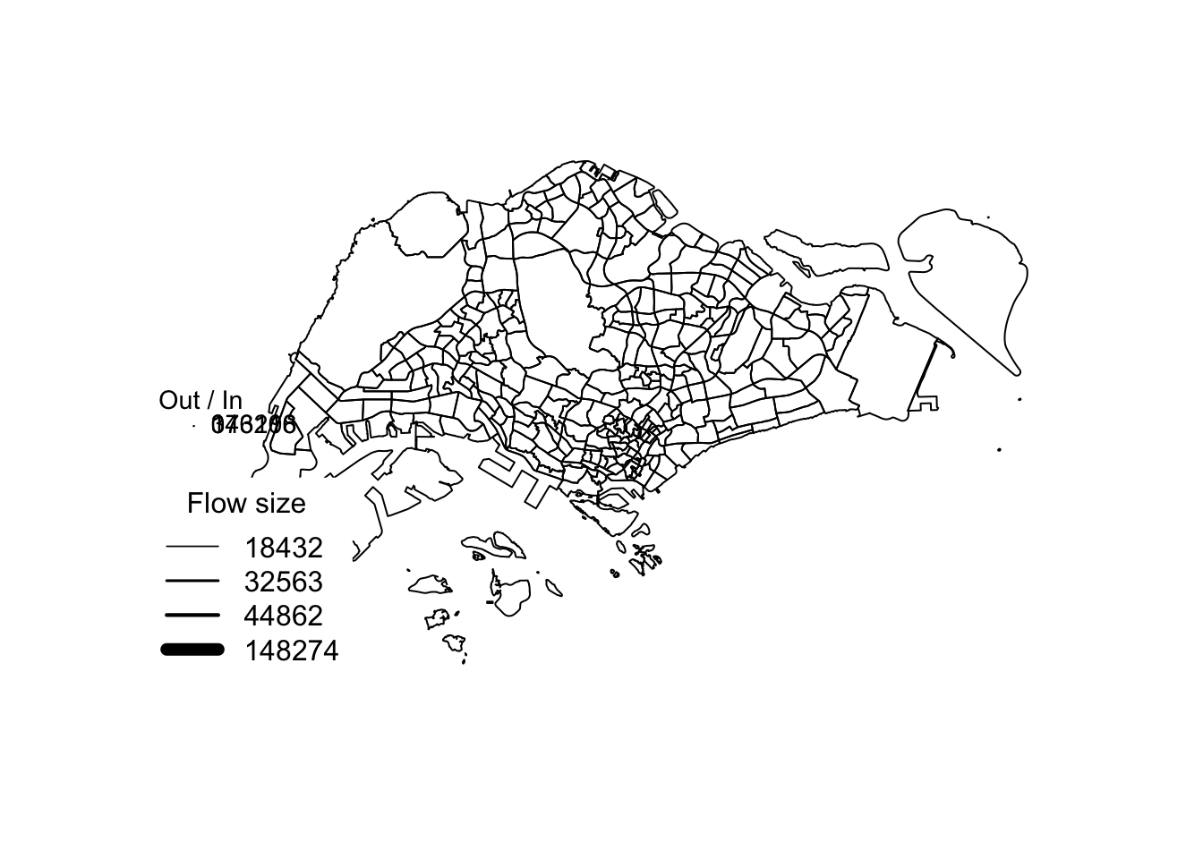
cor_formula <- log(1 + TRIPS) ~
    BUSSTOP_COUNT +
    AGE7_12 +
    AGE13_24 +
    AGE25_64 +
    SCHOOL_COUNT +
    BUSINESS_COUNT +
    RETAILS_COUNT +
    FINSERV_COUNT +
    P_(log(DISTANCE + 1))

cor_mat <- pair_cor(
  mpsz_multi_net,
  spflow_formula = cor_formula,
  add_lags_x = FALSE)

colnames(cor_mat) <- paste0(
  substr(
    colnames(cor_mat),1,3),"...")

cor_image(cor_mat)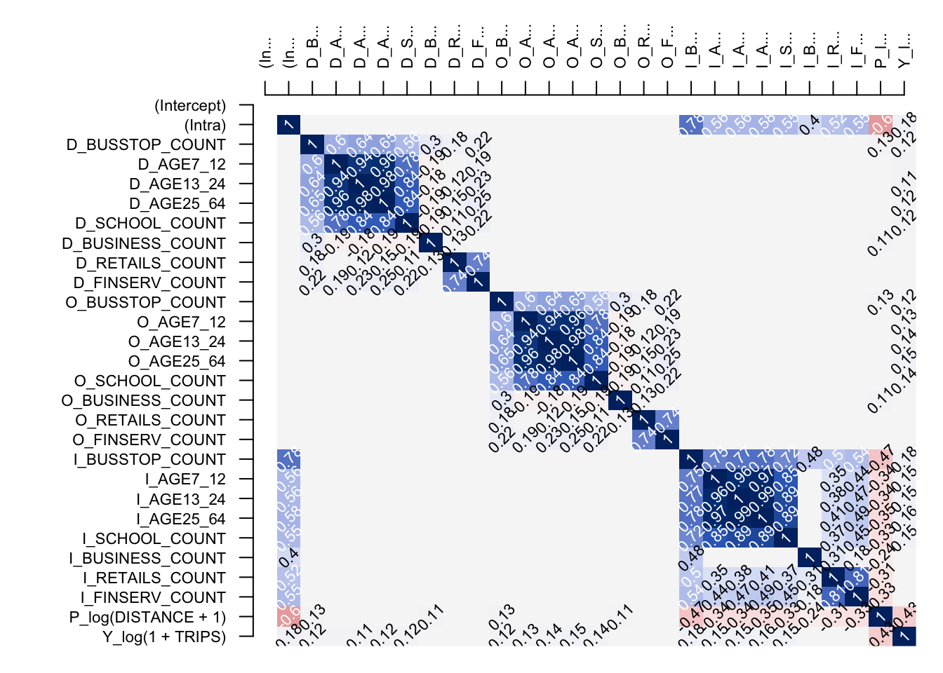
base_model <- spflow(
  spflow_formula = log(1 + TRIPS) ~
    O_(BUSSTOP_COUNT +
         AGE25_64) +
    D_(SCHOOL_COUNT +
    BUSINESS_COUNT +
    RETAILS_COUNT +
    FINSERV_COUNT) +
    P_(log(DISTANCE + 1)),
  spflow_networks = mpsz_multi_net)

base_model
--------------------------------------------------
Spatial interaction model estimated by: MLE
Spatial correlation structure: SDM (model_9)
Dependent variable: log(1 + TRIPS)
--------------------------------------------------
Coefficients:
est sd t.stat p.val
rho_d 0.680 0.004 192.553 0.000
rho_o 0.678 0.004 187.732 0.000
rho_w -0.396 0.006 -65.590 0.000
(Intercept) 0.410 0.065 6.266 0.000
(Intra) 1.313 0.081 16.263 0.000
D_SCHOOL_COUNT 0.017 0.002 7.885 0.000
D_SCHOOL_COUNT.lag1 0.002 0.004 0.551 0.581
D_BUSINESS_COUNT 0.000 0.000 3.015 0.003
D_BUSINESS_COUNT.lag1 0.000 0.000 -0.249 0.804
D_RETAILS_COUNT 0.000 0.000 -0.306 0.759
D_RETAILS_COUNT.lag1 0.000 0.000 0.152 0.880
D_FINSERV_COUNT 0.002 0.000 6.787 0.000
D_FINSERV_COUNT.lag1 -0.002 0.001 -3.767 0.000
O_BUSSTOP_COUNT 0.002 0.000 6.807 0.000
O_BUSSTOP_COUNT.lag1 -0.001 0.000 -2.364 0.018
O_AGE25_64 0.000 0.000 7.336 0.000
O_AGE25_64.lag1 0.000 0.000 -2.797 0.005
P_log(DISTANCE + 1) -0.050 0.007 -6.793 0.000
--------------------------------------------------
R2_corr: 0.6942943
Observations: 97969
Model coherence: Validatedold_par <- par(mfrow = c(1, 3),
mar = c(2,2,2,2))
spflow_moran_plots(base_model)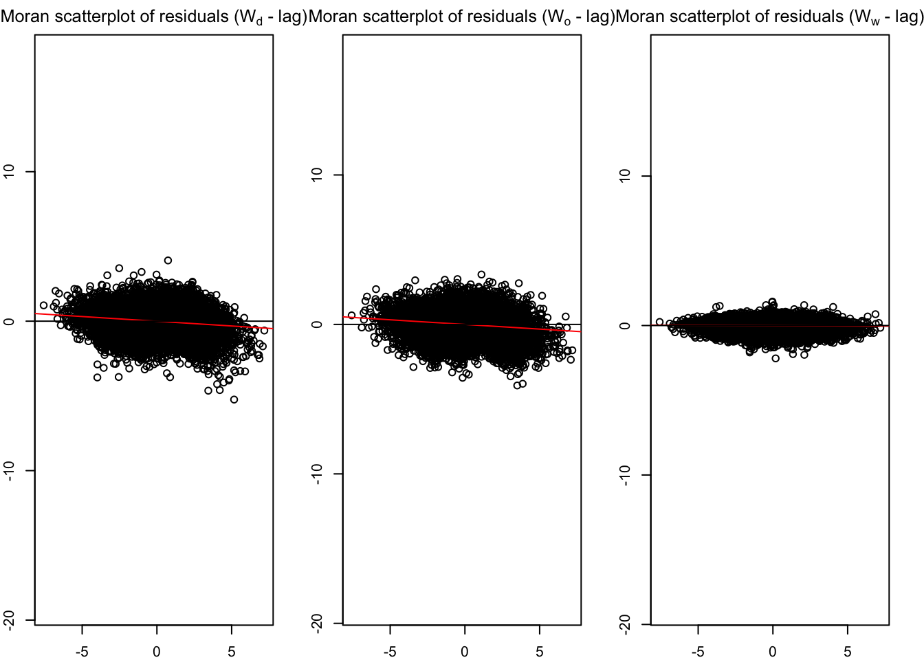
corr_residual <- pair_cor(base_model)
colnames(corr_residual) <- substr(colnames(corr_residual),1,3)
cor_image(corr_residual)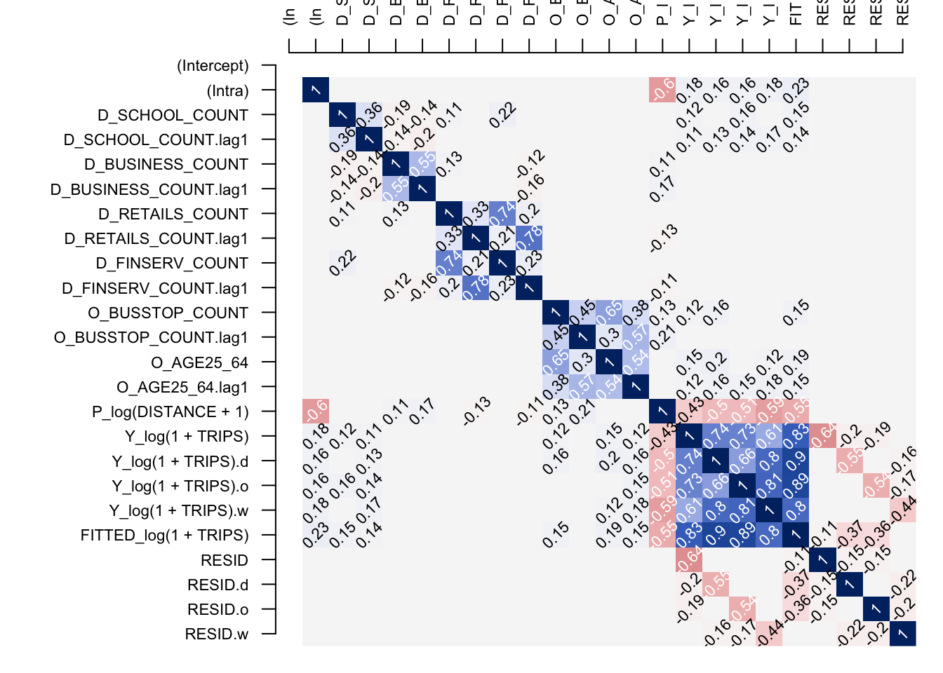
model.df <- as_tibble(base_model@spflow_indicators) %>%
  mutate(FITTED_Y = round(exp(FITTED),0))
mpsz_flow1 <- mpsz_flow %>%
left_join(model.df) %>%
select(1:4,8) %>%
mutate(diff = (FITTED_Y-TRIPS))Joining with `by = join_by(ORIGIN_SZ, DESTIN_SZ)`spflow_formula <- log(1 + TRIPS) ~
O_(BUSSTOP_COUNT +
AGE25_64) +
D_(SCHOOL_COUNT +
BUSINESS_COUNT +
RETAILS_COUNT +
FINSERV_COUNT) +
P_(log(DISTANCE + 1))
model_control <- spflow_control(
estimation_method = "mle",
model = "model_8")
mle_model8 <- spflow(
spflow_formula,
spflow_networks = mpsz_multi_net,
estimation_control = model_control)
mle_model8--------------------------------------------------
Spatial interaction model estimated by: MLE
Spatial correlation structure: SDM (model_8)
Dependent variable: log(1 + TRIPS)
--------------------------------------------------
Coefficients:
est sd t.stat p.val
rho_d 0.689 0.003 196.833 0.000
rho_o 0.687 0.004 192.214 0.000
rho_w -0.473 0.003 -142.469 0.000
(Intercept) 1.086 0.049 22.274 0.000
(Intra) 0.840 0.075 11.255 0.000
D_SCHOOL_COUNT 0.019 0.002 8.896 0.000
D_SCHOOL_COUNT.lag1 0.019 0.004 5.129 0.000
D_BUSINESS_COUNT 0.000 0.000 3.328 0.001
D_BUSINESS_COUNT.lag1 0.000 0.000 1.664 0.096
D_RETAILS_COUNT 0.000 0.000 -0.414 0.679
D_RETAILS_COUNT.lag1 0.000 0.000 -0.171 0.864
D_FINSERV_COUNT 0.002 0.000 6.150 0.000
D_FINSERV_COUNT.lag1 -0.003 0.001 -4.601 0.000
O_BUSSTOP_COUNT 0.003 0.000 7.676 0.000
O_BUSSTOP_COUNT.lag1 0.000 0.000 0.552 0.581
O_AGE25_64 0.000 0.000 6.870 0.000
O_AGE25_64.lag1 0.000 0.000 -0.462 0.644
P_log(DISTANCE + 1) -0.125 0.005 -22.865 0.000
--------------------------------------------------
R2_corr: 0.6965976
Observations: 97969
Model coherence: Validatedold_par <- par(mfrow = c(1, 3),
mar = c(2,2,2,2))
spflow_moran_plots(mle_model8)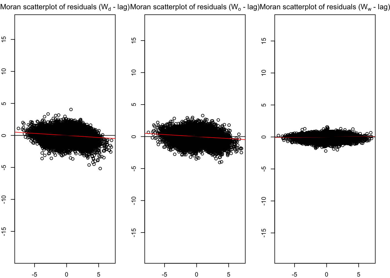
par(old_par)