pacman::p_load(sf, sfdep, tmap, tidyverse, knitr, ggplot2, mapview, spdep, dplyr, plotly, Kendall)take home exercise 1: Geospatial Analytics for Public Good
Overview
With the advancement of our technology, GPS and RFID systems are now installed in our vehicles, particularly in public buses equipped with smart cards and GPS that collect extensive data on routes and passenger volumes. Analyzing these mobility data helps us gain a deeper understanding of people’s lifestyles and habits. This understanding enables us to better manage urban systems and provides valuable information to both private and public sectors in urban transport services, assisting in making informed decisions to gain a competitive edge.
Objective
The objective of our study is to uncover the spatial and spatio-temporal mobility patterns of public bus passengers in Singapore by applying appropriate Local Indicators of Spatial Association (LISA) and Emerging Hot Spot Analysis (EHSA) through the method of Exploratory Spatial Data Analysis (ESDA).
Analytical
Get Started Setting the Analytical Tools The code chunk below installs and loads sf, spdep, tmap, tidyverse, patchwork packages into R environment. pacman() is a R package management tool.
Data Preparation Aspatial data Passenger Volume by Origin Destination Bus Stops privoded by LTADataMall
Geospatial data * Bus Stop Location from LTA DataMall. It privodes the bus stop code(identifier) and location coordinates. * hexagon, a hexagon layer of 250m (this distance is the perpendicular distance between the centre of the hexagon and its edges.)
A quick look at the busstop within an R object
glimpse(busstop)Rows: 5,161
Columns: 4
$ BUS_STOP_N <chr> "22069", "32071", "44331", "96081", "11561", "66191", "2338…
$ BUS_ROOF_N <chr> "B06", "B23", "B01", "B05", "B05", "B03", "B02A", "B02", "B…
$ LOC_DESC <chr> "OPP CEVA LOGISTICS", "AFT TRACK 13", "BLK 239", "GRACE IND…
$ geometry <POINT [m]> POINT (13576.31 32883.65), POINT (13228.59 44206.38),…Read the busstops
odbus <- read_csv("data/aspatial/origin_destination_bus_202308.csv")Rows: 5709512 Columns: 7
── Column specification ────────────────────────────────────────────────────────
Delimiter: ","
chr (5): YEAR_MONTH, DAY_TYPE, PT_TYPE, ORIGIN_PT_CODE, DESTINATION_PT_CODE
dbl (2): TIME_PER_HOUR, TOTAL_TRIPS
ℹ Use `spec()` to retrieve the full column specification for this data.
ℹ Specify the column types or set `show_col_types = FALSE` to quiet this message.Convert to the factor
odbus$ORIGIN_PT_CODE <- as.factor(odbus$ORIGIN_PT_CODE)
odbus$DESTINATION_PT_CODE <- as.factor(odbus$ORIGIN_PT_CODE)
A quick look at odbus
glimpse(odbus)Rows: 5,709,512
Columns: 7
$ YEAR_MONTH <chr> "2023-08", "2023-08", "2023-08", "2023-08", "2023-…
$ DAY_TYPE <chr> "WEEKDAY", "WEEKENDS/HOLIDAY", "WEEKENDS/HOLIDAY",…
$ TIME_PER_HOUR <dbl> 16, 16, 14, 14, 17, 17, 17, 17, 7, 17, 14, 10, 10,…
$ PT_TYPE <chr> "BUS", "BUS", "BUS", "BUS", "BUS", "BUS", "BUS", "…
$ ORIGIN_PT_CODE <fct> 04168, 04168, 80119, 80119, 44069, 44069, 20281, 2…
$ DESTINATION_PT_CODE <fct> 04168, 04168, 80119, 80119, 44069, 44069, 20281, 2…
$ TOTAL_TRIPS <dbl> 7, 2, 3, 10, 5, 4, 3, 22, 3, 3, 7, 1, 3, 1, 3, 1, …Geovisuallisation and Analysis the peak time – weekday morning, weekday afternoon, weekend morning and weekend evening.
weekdaymorning6_9 <- odbus %>%
  filter(DAY_TYPE == "WEEKDAY") %>%
  filter(TIME_PER_HOUR >= 6 &
           TIME_PER_HOUR <= 9) %>%
  group_by(ORIGIN_PT_CODE) %>%
summarise(TRIPS = sum(TOTAL_TRIPS))kable(head(weekdaymorning6_9))| ORIGIN_PT_CODE | TRIPS |
|---|---|
| 01012 | 1973 |
| 01013 | 952 |
| 01019 | 1789 |
| 01029 | 2561 |
| 01039 | 2938 |
| 01059 | 1651 |
weekdayafternoon17_20 <- odbus %>%
  filter(DAY_TYPE == "WEEKDAY") %>%
  filter(TIME_PER_HOUR >= 17 &
           TIME_PER_HOUR <= 20) %>%
  group_by(ORIGIN_PT_CODE) %>%
summarise(TRIPS = sum(TOTAL_TRIPS))kable(head(weekdayafternoon17_20))| ORIGIN_PT_CODE | TRIPS |
|---|---|
| 01012 | 8448 |
| 01013 | 7328 |
| 01019 | 3608 |
| 01029 | 9317 |
| 01039 | 12937 |
| 01059 | 2133 |
weekendmorning11_14 <- odbus %>%
  filter(DAY_TYPE == "WEEKENDS/HOLIDAY") %>%
  filter(TIME_PER_HOUR >= 11 &
           TIME_PER_HOUR <= 14) %>%
  group_by(ORIGIN_PT_CODE) %>%
summarise(TRIPS = sum(TOTAL_TRIPS))kable(head(weekendmorning11_14))| ORIGIN_PT_CODE | TRIPS |
|---|---|
| 01012 | 2273 |
| 01013 | 1697 |
| 01019 | 1511 |
| 01029 | 3272 |
| 01039 | 5424 |
| 01059 | 1062 |
weekendevening16_19 <- odbus %>%
  filter(DAY_TYPE == "WEEKENDS/HOLIDAY") %>%
  filter(TIME_PER_HOUR >= 16 &
           TIME_PER_HOUR <= 19) %>%
  group_by(ORIGIN_PT_CODE) %>%
summarise(TRIPS = sum(TOTAL_TRIPS))kable(head(weekendevening16_19))| ORIGIN_PT_CODE | TRIPS |
|---|---|
| 01012 | 3208 |
| 01013 | 2796 |
| 01019 | 1623 |
| 01029 | 4244 |
| 01039 | 7403 |
| 01059 | 1190 |
weekdaymorning6_9_summarized <- weekdaymorning6_9 %>%
  group_by(ORIGIN_PT_CODE) %>%
  summarise(TotalTrips = sum(TRIPS))
weekdayafternoon17_20_summarized <- weekdayafternoon17_20 %>%
group_by(ORIGIN_PT_CODE) %>%
summarise(TotalTrips = sum(TRIPS))weekendmorning11_14_summarized <- weekendmorning11_14 %>%
group_by(ORIGIN_PT_CODE) %>%
summarise(TotalTrips = sum(TRIPS))weekendevening16_19_summarized <- weekendevening16_19 %>%
group_by(ORIGIN_PT_CODE) %>%
summarise(TotalTrips = sum(TRIPS))Create the rds file
if (!dir.exists("data/rds")) {
  dir.create("data/rds", recursive = TRUE)
}
Save the 4 peak time period
write_rds(weekdaymorning6_9_summarized, "data/rds/weekdaymorning6_9_summarized.rds")
write_rds(weekdayafternoon17_20_summarized, "data/rds/weekdayafternoon17_20_summarized.rds")
write_rds(weekendmorning11_14_summarized, "data/rds/weekendmorning11_14_summarized.rds")
write_rds(weekendevening16_19_summarized, "data/rds/weekendevening16_19_summarized.rds")
weekdaymorning6_9_summarized <- read_rds("data/rds/weekdaymorning6_9_summarized.rds")
weekdayafternoon17_20_summviewarized <- read_rds("data/rds/weekdayafternoon17_20_summarized.rds")
weekendmorning11_14_summarized <- read_rds("data/rds/weekendmorning11_14_summarized.rds")
weekendevening16_19_summarized <- read_rds("data/rds/weekendevening16_19_summarized.rds")Left join busstop and peak time
busstops_weekday_morning <- left_join(busstop, weekdaymorning6_9_summarized, by = c("BUS_STOP_N" = "ORIGIN_PT_CODE"))
busstops_weekday_afternoon <- left_join(busstop, weekdayafternoon17_20_summarized, by = c("BUS_STOP_N" = "ORIGIN_PT_CODE"))
busstops_weekend_morning <- left_join(busstop, weekendmorning11_14_summarized, by = c("BUS_STOP_N" = "ORIGIN_PT_CODE"))
busstops_weekend_evening <- left_join(busstop, weekendevening16_19_summarized, by = c("BUS_STOP_N" = "ORIGIN_PT_CODE"))
Draw 4 Hexagon
hexagon_grid_weekday_morning <- st_make_grid(busstops_weekday_morning, cellsize = c(250, 250), what = "polygons", square = FALSE)
hexagon_grid_sf_weekday_morning <- st_sf(geometry = hexagon_grid_weekday_morning) %>%
  mutate(grid_id = 1:length(lengths(hexagon_grid_weekday_morning)))
hexagon_grid_weekday_afternoon <- st_make_grid(busstops_weekday_afternoon, cellsize = c(250, 250), what = "polygons", square = FALSE)
hexagon_grid_sf_weekday_afternoon <- st_sf(geometry = hexagon_grid_weekday_afternoon) %>%
mutate(grid_id = 1:length(lengths(hexagon_grid_weekday_afternoon)))hexagon_grid_weekend_morning <- st_make_grid(busstops_weekend_morning, cellsize = c(250, 250), what = "polygons", square = FALSE)
hexagon_grid_sf_weekend_morning <- st_sf(geometry = hexagon_grid_weekend_morning) %>%
mutate(grid_id = 1:length(lengths(hexagon_grid_weekend_morning)))hexagon_grid_weekend_evening <- st_make_grid(busstops_weekend_evening, cellsize = c(250, 250), what = "polygons", square = FALSE)
hexagon_grid_sf_weekend_evening<- st_sf(geometry = hexagon_grid_weekend_evening) %>%
mutate(grid_id = 1:length(lengths(hexagon_grid_weekend_evening)))Show busstop map
hexagon_grid_weekday_morning <- st_make_grid(busstops_weekday_morning, cellsize = c(250, 250), what = "polygons", square = FALSE)
hexagon_grid_sf_weekday_morning <- st_sf(geometry = hexagon_grid_weekday_morning) %>%
  mutate(grid_id = 1:length(lengths(hexagon_grid_weekday_morning)))
hexagon_grid_sf_weekday_morning$n_colli = lengths(st_intersects(hexagon_grid_sf_weekday_morning, busstops_weekday_morning))
hexagon_count_busstops_weekday_morning = filter(hexagon_grid_sf_weekday_morning, n_colli > 0)
map_honeycomb <- tm_shape(hexagon_count_busstops_weekday_morning) +
tm_fill(
col = "n_colli",
palette = "Reds",
style = "cont",
title = "Number of busstops",
id = "grid_id",
showNA = FALSE,
alpha = 0.6,
popup.vars = c(
"Number of busstops: " = "n_colli"
),
popup.format = list(
n_colli = list(format = "f", digits = 0)
)
) +
tm_borders(col = "grey40", lwd = 0.7)
map_honeycomb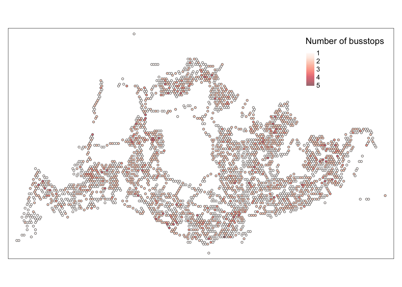
tmap_mode("plot")tmap mode set to plottingDraw 4 peak time maps
intersects_list_morning <- st_intersects(hexagon_grid_sf_weekday_morning, busstops_weekday_morning)
total_trips_morning <- purrr::map_dbl(intersects_list_morning, ~sum(busstops_weekday_morning$TotalTrips[.x], na.rm = TRUE))
hexagon_grid_sf_weekday_morning$TotalTrips <- total_trips_morning
hexagon_count_totaltrips_morning <- hexagon_grid_sf_weekday_morning %>%
  filter(TotalTrips > 0)
map_honeycomb_morning <- tm_shape(hexagon_count_totaltrips_morning) +
tm_fill(
col = "TotalTrips",
palette = "Reds",
style = "cont",
title = "Number of TotalTrips - Morning",
showNA = FALSE,
alpha = 0.6,
popup.vars = c("Number of TotalTrips: " = "TotalTrips"),
popup.format = list(TotalTrips = list(format = "f", digits = 0))
) +
tm_borders(col = "grey40", lwd = 0.7)
map_honeycomb_morning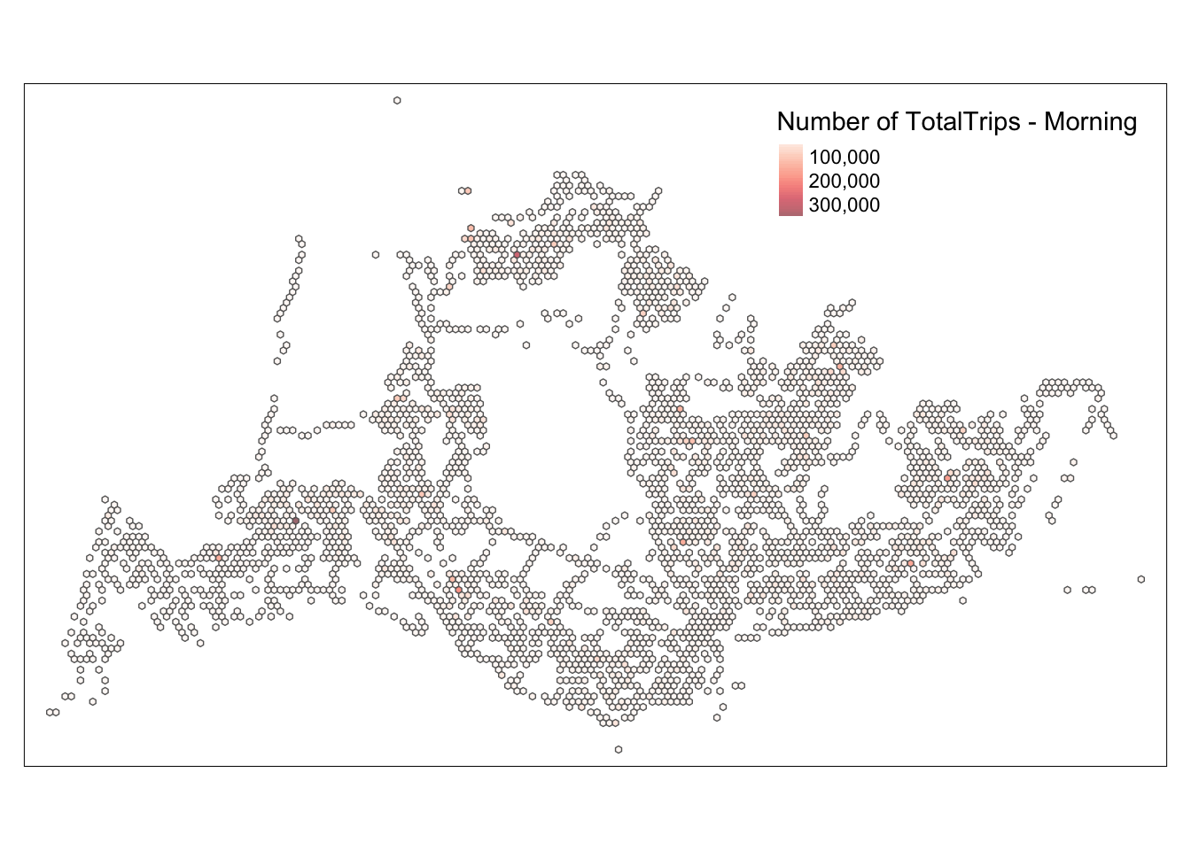
intersects_list_afternoon <- st_intersects(hexagon_grid_sf_weekday_afternoon, busstops_weekday_afternoon)
total_trips_afternoon <- purrr::map_dbl(intersects_list_afternoon, ~sum(busstops_weekday_afternoon$TotalTrips[.x], na.rm = TRUE))
hexagon_grid_sf_weekday_afternoon$TotalTrips <- total_trips_afternoon
hexagon_count_totaltrips_afternoon <- hexagon_grid_sf_weekday_afternoon %>%
  filter(TotalTrips > 0)
map_honeycomb_afternoon <- tm_shape(hexagon_count_totaltrips_afternoon) +
tm_fill(
col = "TotalTrips",
palette = "Reds",
style = "cont",
title = "Number of TotalTrips - Afternoon",
showNA = FALSE,
alpha = 0.6,
popup.vars = c("Number of TotalTrips: " = "TotalTrips"),
popup.format = list(TotalTrips = list(format = "f", digits = 0))
) +
tm_borders(col = "grey40", lwd = 0.7)
map_honeycomb_afternoon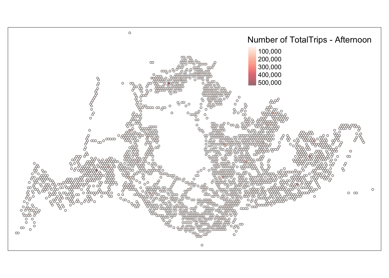
intersects_list_weekend_morning <- st_intersects(hexagon_grid_sf_weekend_morning, busstops_weekend_morning)
total_trips_weekend_morning <- purrr::map_dbl(intersects_list_weekend_morning, ~sum(busstops_weekend_morning$TotalTrips[.x], na.rm = TRUE))
hexagon_grid_sf_weekend_morning$TotalTrips <- total_trips_weekend_morning
hexagon_count_totaltrips_weekend_morning <- hexagon_grid_sf_weekend_morning %>%
  filter(TotalTrips > 0)
map_honeycomb_weekend_morning <- tm_shape(hexagon_count_totaltrips_weekend_morning) +
tm_fill(
col = "TotalTrips",
palette = "Reds",
style = "cont",
title = "Number of TotalTrips - Weekend Morning",
showNA = FALSE,
alpha = 0.6,
popup.vars = c("Number of TotalTrips: " = "TotalTrips"),
popup.format = list(TotalTrips = list(format = "f", digits = 0))
) +
tm_borders(col = "grey40", lwd = 0.7)
map_honeycomb_weekend_morning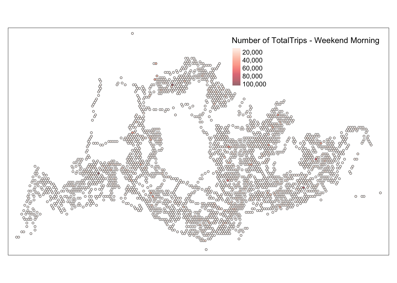
intersects_list_weekend_evening <- st_intersects(hexagon_grid_sf_weekend_evening, busstops_weekend_evening)
total_trips_weekend_evening <- purrr::map_dbl(intersects_list_weekend_evening, ~sum(busstops_weekend_evening$TotalTrips[.x], na.rm = TRUE))
hexagon_grid_sf_weekend_evening$TotalTrips <- total_trips_weekend_evening
hexagon_count_totaltrips_weekend_evening <- hexagon_grid_sf_weekend_evening %>%
  filter(TotalTrips > 0)
map_honeycomb_weekend_evening <- tm_shape(hexagon_count_totaltrips_weekend_evening)+
tm_fill(
col = "TotalTrips",
palette = "Reds",
style = "cont",
title = "Number of TotalTrips - Weekend Evening",
showNA = FALSE,
alpha = 0.6,
popup.vars = c("Number of TotalTrips: " = "TotalTrips"),
popup.format = list(TotalTrips = list(format = "f", digits = 0))
) +
tm_borders(col = "grey40", lwd = 0.7)
map_honeycomb_weekend_evening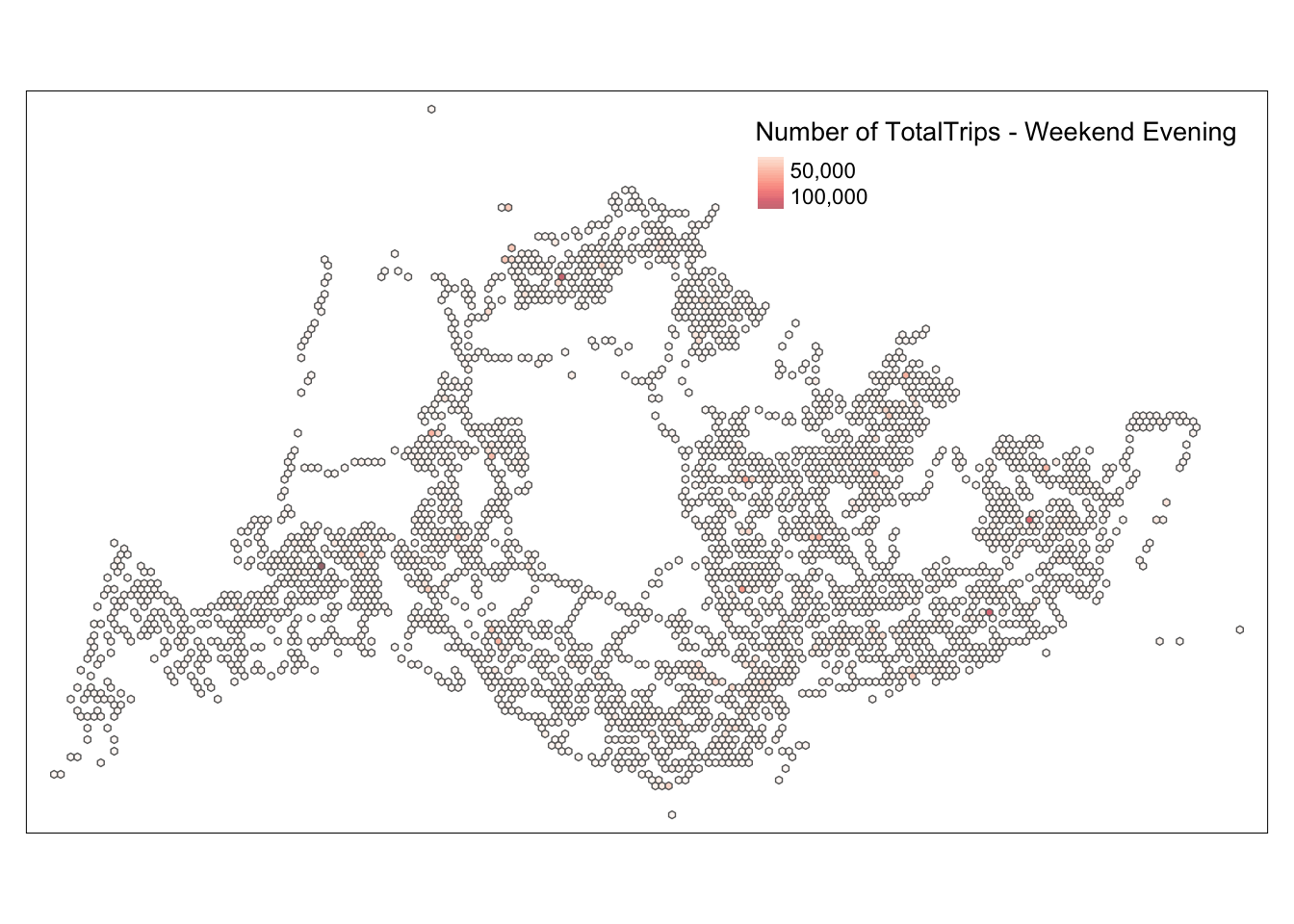
tmap_mode("plot")tmap mode set to plottingConclusion
Based on this map, we can see that the traffic during the usual morning and evening peak hours and the weekend peak hours are quite similar. By comparing the entire scenario, we can deduce that the design of the bus stops is very consistent with the peak travel times. From the map, we can also identify a few particular points, such as 4982 and 5478, where the number of people is relatively high at all four time points. The map only provides some general and rough information; we need a more detailed analysis to assess whether our bus route design is reasonable.
Analysis Lisa
LISA peak time weekday morning
wm_q <- hexagon_count_totaltrips_morning %>%
  mutate(nb = st_knn(geometry,
                     k=8),
         wt = st_weights(nb),
               .before = 1)
! Polygon provided. Using point on surface.moranI <- global_moran(wm_q$TotalTrips,
wm_q$nb,
wm_q$wt)
glimpse(moranI)List of 2
$ I: num 0.125
$ K: num 130global_moran_test(wm_q$TotalTrips,
wm_q$nb,
wm_q$wt)
    Moran I test under randomisation

data:  x
weights: listw

Moran I statistic standard deviate = 14.71, p-value < 2.2e-16
alternative hypothesis: greater
sample estimates:
Moran I statistic       Expectation          Variance
1.247405e-01 -3.282994e-04 7.228939e-05 set.seed(1234)global_moran_perm(wm_q$TotalTrips,
wm_q$nb,
wm_q$wt,
nsim = 99)
    Monte-Carlo simulation of Moran I

data:  x
weights: listw
number of simulations + 1: 100

statistic = 0.12474, observed rank = 100, p-value < 2.2e-16
alternative hypothesis: two.sided
lisa <- wm_q %>%
mutate(local_moran = local_moran(
TotalTrips, nb, wt, nsim = 99),
.before = 1) %>%
unnest(local_moran)tmap_mode("plot")tmap mode set to plottingtm_shape(lisa) +
tm_fill("ii") +
tm_borders(alpha = 0.5) +
tm_view(set.zoom.limits = c(6,8)) +
tm_layout(main.title = "local Moran's I of Totaltrips",
main.title.size = 0.8)Variable(s) "ii" contains positive and negative values, so midpoint is set to 0. Set midpoint = NA to show the full spectrum of the color palette.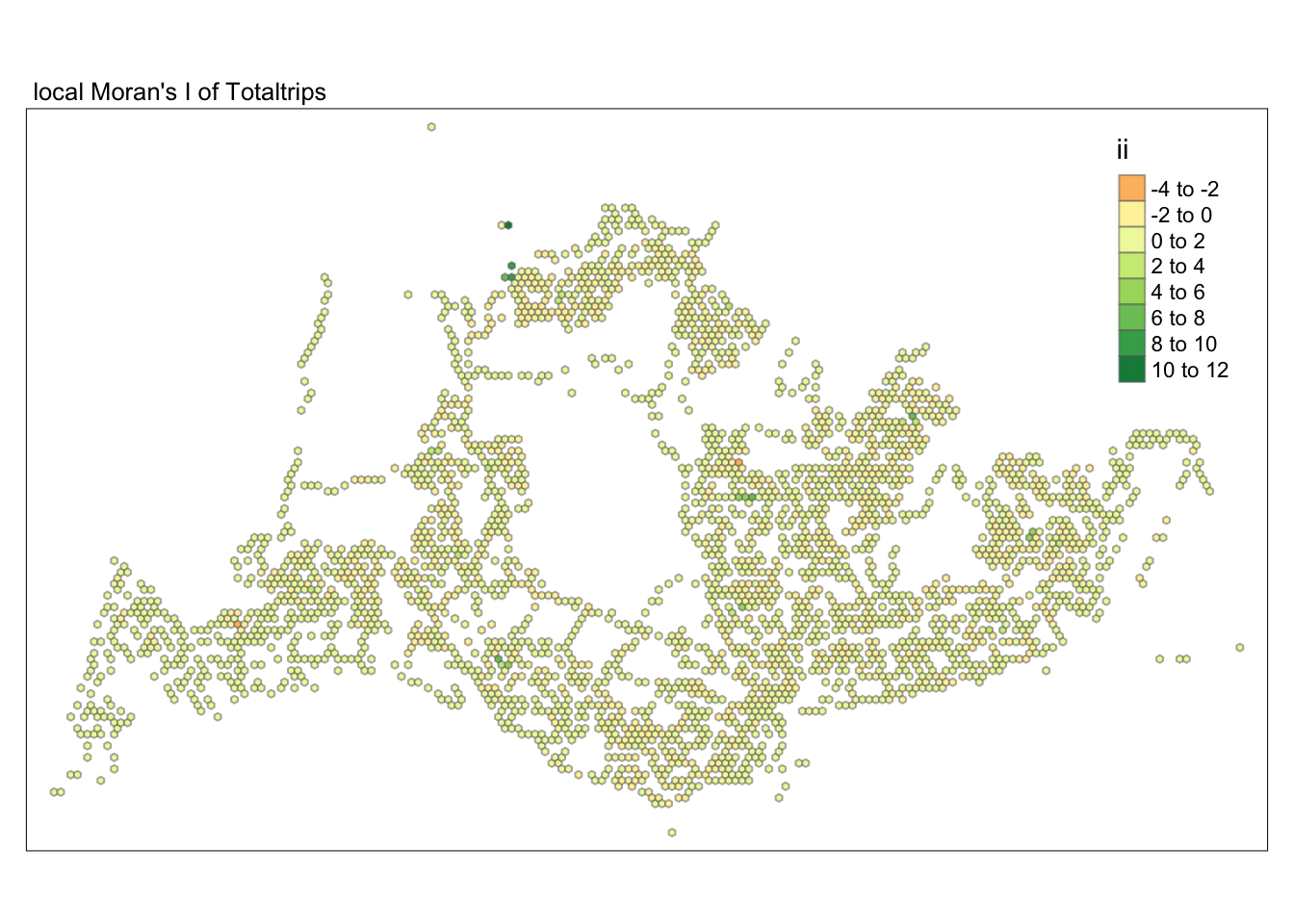
tmap_mode("plot")tmap mode set to plottingtm_shape(lisa) +
tm_fill("p_ii_sim") +
tm_borders(alpha = 0.5) +
tm_layout(main.title = "p-value of local Moran's I",
main.title.size = 0.8)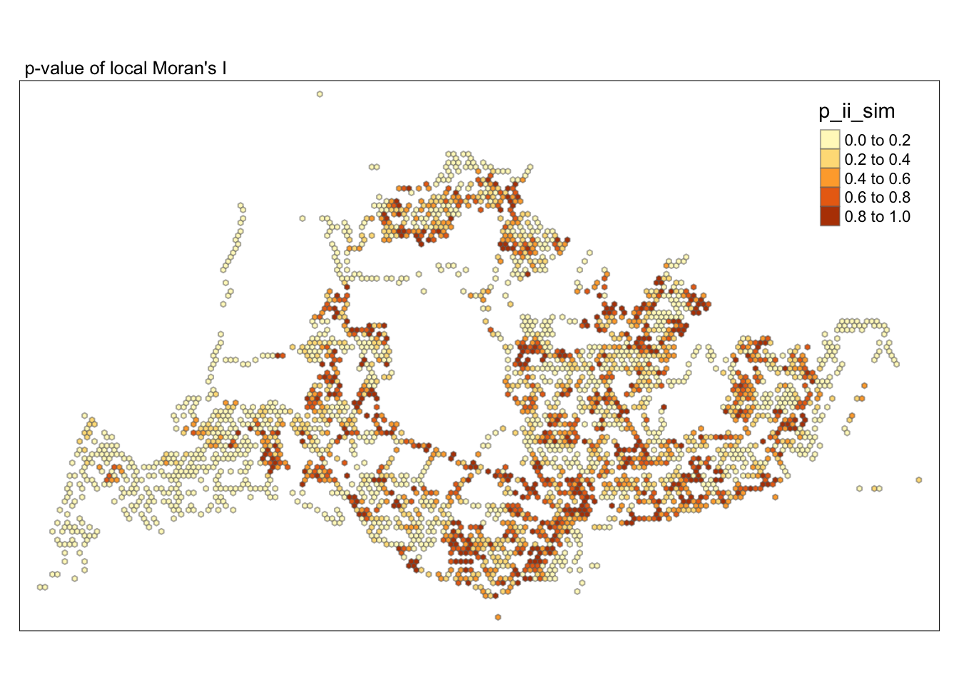
tmap_mode("plot")tmap mode set to plottingmap1 <- tm_shape(lisa) +
tm_fill("ii") +
tm_borders(alpha = 0.5) +
tm_view(set.zoom.limits = c(6,8)) +
tm_layout(main.title = "local Moran's I of Totaltrips",
main.title.size = 0.8)
map2 <- tm_shape(lisa) +
tm_fill("p_ii_sim",
breaks = c(0, 0.001, 0.01, 0.05, 1),
labels = c("0.001", "0.01", "0.05", "Not sig")) +
tm_borders(alpha = 0.5) +
tm_layout(main.title = "p-value of local Moran's I",
main.title.size = 0.8)
tmap_arrange(map1, map2, ncol = 2)Variable(s) "ii" contains positive and negative values, so midpoint is set to 0. Set midpoint = NA to show the full spectrum of the color palette.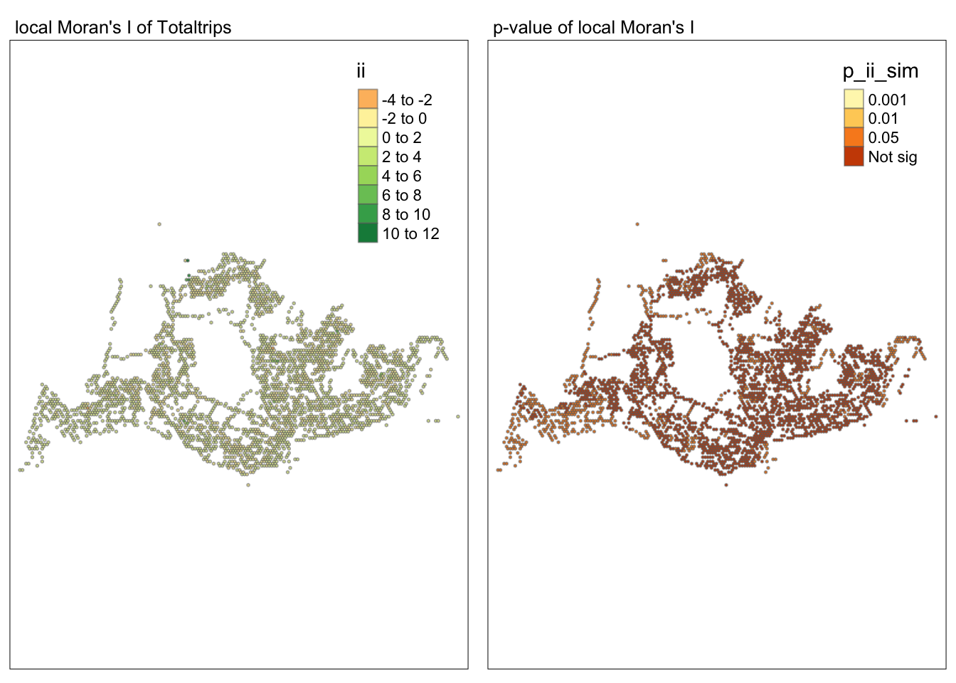
lisa_sig <- lisa  %>%
  filter(p_ii_sim < 0.05)
tmap_mode("plot")
tmap mode set to plottingtm_shape(lisa) +
tm_polygons() +
tm_borders(alpha = 0.5) +
tm_shape(lisa_sig) +
tm_fill("mean") +
tm_borders(alpha = 0.4)Warning: One tm layer group has duplicated layer types, which are omitted. To
draw multiple layers of the same type, use multiple layer groups (i.e. specify
tm_shape prior to each of them).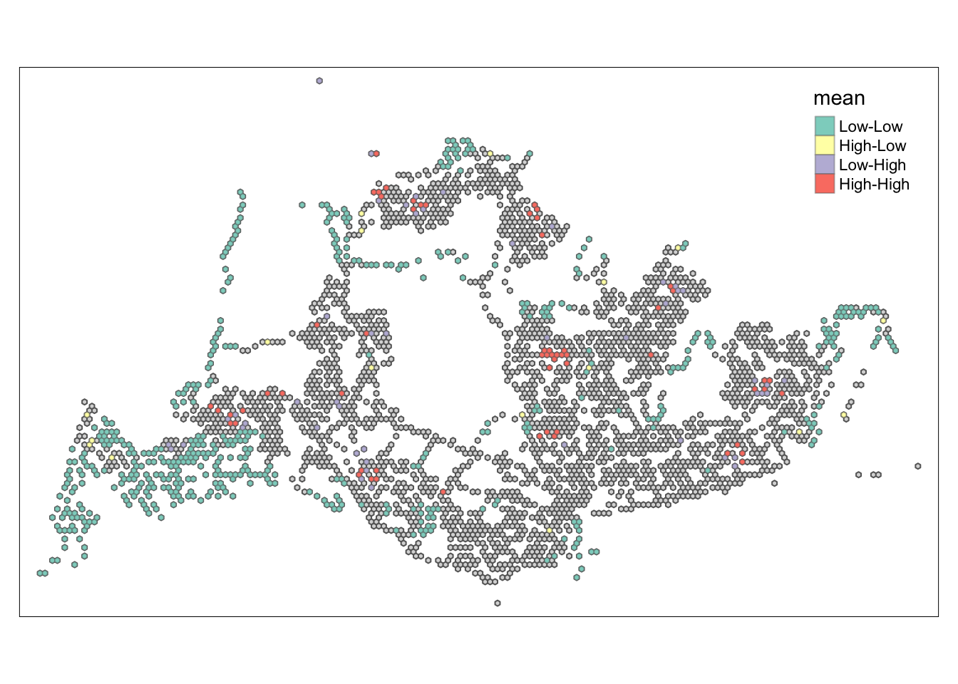
LISA peak time weekday afternoon
wm_q <- hexagon_count_totaltrips_afternoon %>%
  mutate(nb = st_knn(geometry,
                     k=8),
         wt = st_weights(nb),
               .before = 1)
! Polygon provided. Using point on surface.moranI <- global_moran(wm_q$TotalTrips,
wm_q$nb,
wm_q$wt)
glimpse(moranI)List of 2
$ I: num 0.0595
$ K: num 214global_moran_test(wm_q$TotalTrips,
wm_q$nb,
wm_q$wt)
    Moran I test under randomisation

data:  x
weights: listw

Moran I statistic standard deviate = 7.1461, p-value = 4.462e-13
alternative hypothesis: greater
sample estimates:
Moran I statistic       Expectation          Variance
5.950141e-02 -3.275467e-04 7.009368e-05 set.seed(1234)global_moran_perm(wm_q$TotalTrips,
wm_q$nb,
wm_q$wt,
nsim = 99)
    Monte-Carlo simulation of Moran I

data:  x
weights: listw
number of simulations + 1: 100

statistic = 0.059501, observed rank = 100, p-value < 2.2e-16
alternative hypothesis: two.sided
lisa <- wm_q %>%
mutate(local_moran = local_moran(
TotalTrips, nb, wt, nsim = 99),
.before = 1) %>%
unnest(local_moran)tmap_mode("plot")tmap mode set to plottingtm_shape(lisa) +
tm_fill("ii") +
tm_borders(alpha = 0.5) +
tm_view(set.zoom.limits = c(6,8)) +
tm_layout(main.title = "local Moran's I of Totaltrips",
main.title.size = 0.8)Variable(s) "ii" contains positive and negative values, so midpoint is set to 0. Set midpoint = NA to show the full spectrum of the color palette.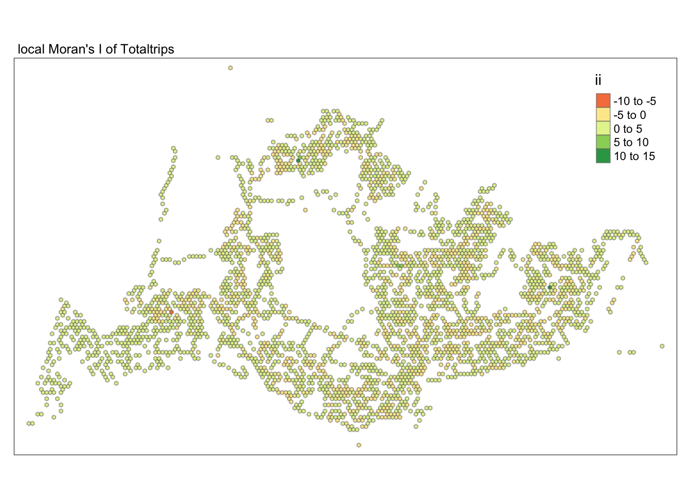
tmap_mode("plot")tmap mode set to plottingtm_shape(lisa) +
tm_fill("p_ii_sim") +
tm_borders(alpha = 0.5) +
tm_layout(main.title = "p-value of local Moran's I",
main.title.size = 0.8)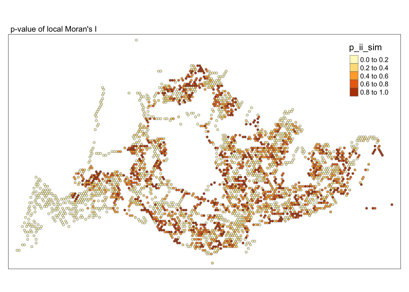
tmap_mode("plot")tmap mode set to plottingmap1 <- tm_shape(lisa) +
tm_fill("ii") +
tm_borders(alpha = 0.5) +
tm_view(set.zoom.limits = c(6,8)) +
tm_layout(main.title = "local Moran's I of Totaltrips",
main.title.size = 0.8)
map2 <- tm_shape(lisa) +
tm_fill("p_ii_sim",
breaks = c(0, 0.001, 0.01, 0.05, 1),
labels = c("0.001", "0.01", "0.05", "Not sig")) +
tm_borders(alpha = 0.5) +
tm_layout(main.title = "p-value of local Moran's I",
main.title.size = 0.8)
tmap_arrange(map1, map2, ncol = 2)Variable(s) "ii" contains positive and negative values, so midpoint is set to 0. Set midpoint = NA to show the full spectrum of the color palette.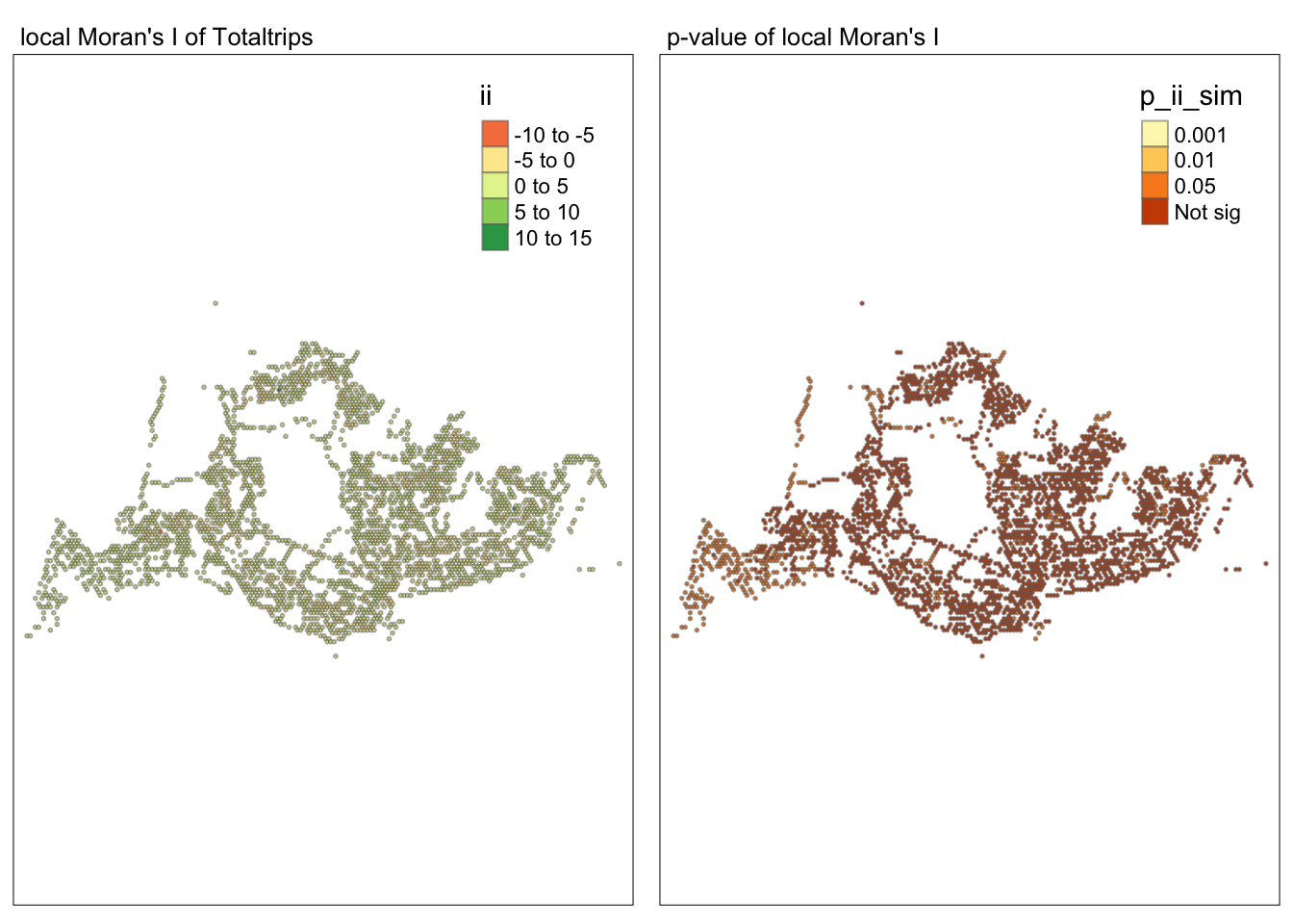
lisa_sig <- lisa  %>%
  filter(p_ii_sim < 0.05)
tmap_mode("plot")
tmap mode set to plottingtm_shape(lisa) +
tm_polygons() +
tm_borders(alpha = 0.5) +
tm_shape(lisa_sig) +
tm_fill("mean") +
tm_borders(alpha = 0.4)Warning: One tm layer group has duplicated layer types, which are omitted. To
draw multiple layers of the same type, use multiple layer groups (i.e. specify
tm_shape prior to each of them).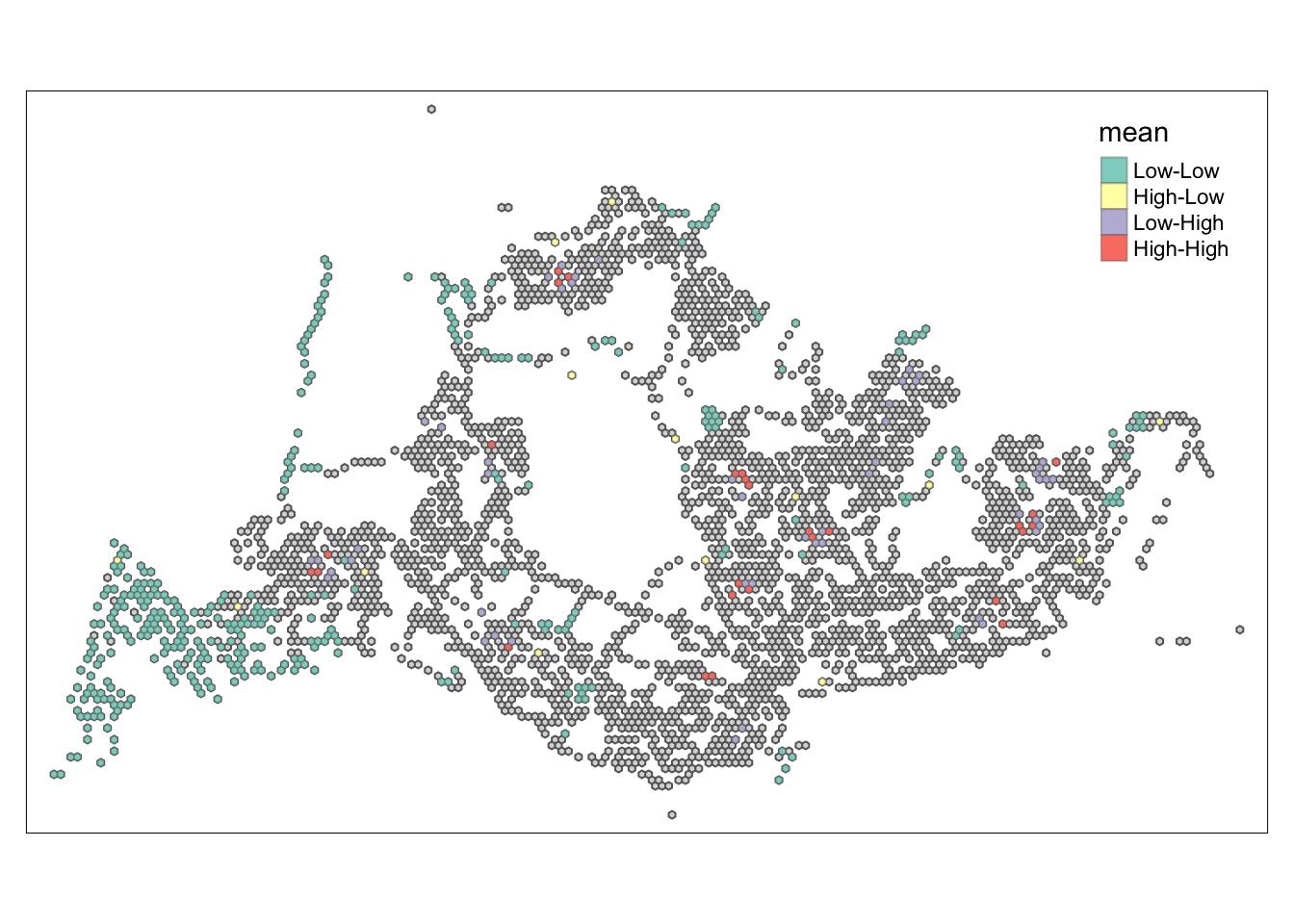
LISA peak time weekend morning
wm_q <- hexagon_count_totaltrips_weekend_morning %>%
  mutate(nb = st_knn(geometry,
                     k=8),
         wt = st_weights(nb),
               .before = 1)
! Polygon provided. Using point on surface.moranI <- global_moran(wm_q$TotalTrips,
wm_q$nb,
wm_q$wt)
glimpse(moranI)List of 2
$ I: num 0.106
$ K: num 131global_moran_test(wm_q$TotalTrips,
wm_q$nb,
wm_q$wt)
    Moran I test under randomisation

data:  x
weights: listw

Moran I statistic standard deviate = 12.532, p-value < 2.2e-16
alternative hypothesis: greater
sample estimates:
Moran I statistic       Expectation          Variance
1.061289e-01 -3.279764e-04 7.215773e-05 set.seed(1234)global_moran_perm(wm_q$TotalTrips,
wm_q$nb,
wm_q$wt,
nsim = 99)
    Monte-Carlo simulation of Moran I

data:  x
weights: listw
number of simulations + 1: 100

statistic = 0.10613, observed rank = 100, p-value < 2.2e-16
alternative hypothesis: two.sided
lisa <- wm_q %>%
mutate(local_moran = local_moran(
TotalTrips, nb, wt, nsim = 99),
.before = 1) %>%
unnest(local_moran)tmap_mode("plot")tmap mode set to plottingtm_shape(lisa) +
tm_fill("ii") +
tm_borders(alpha = 0.5) +
tm_view(set.zoom.limits = c(6,8)) +
tm_layout(main.title = "local Moran's I of Totaltrips",
main.title.size = 0.8)Variable(s) "ii" contains positive and negative values, so midpoint is set to 0. Set midpoint = NA to show the full spectrum of the color palette.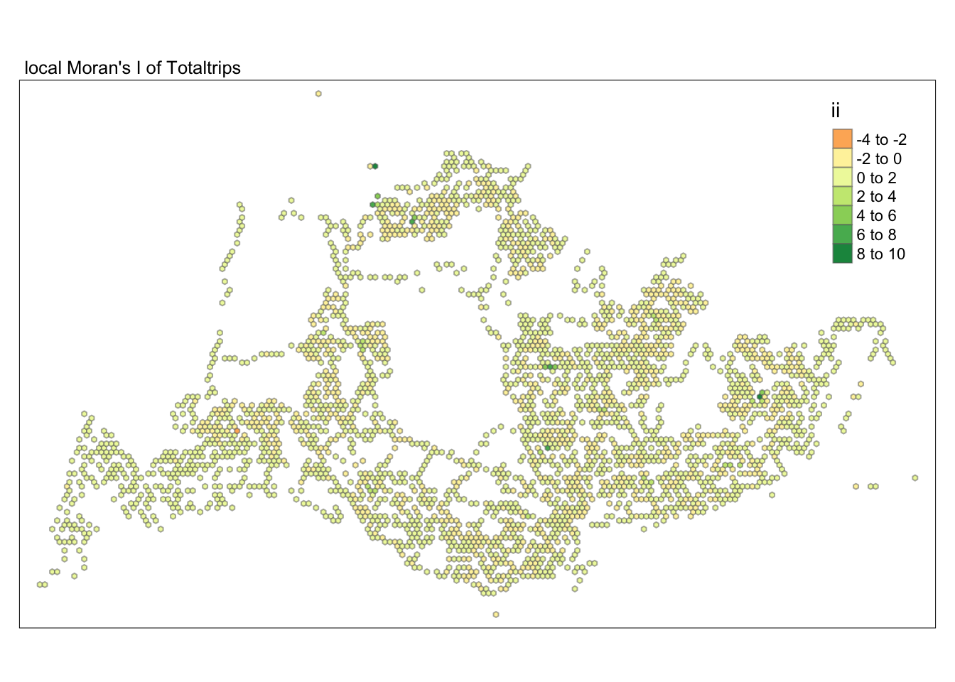
tmap_mode("plot")tmap mode set to plottingtm_shape(lisa) +
tm_fill("p_ii_sim") +
tm_borders(alpha = 0.5) +
tm_layout(main.title = "p-value of local Moran's I",
main.title.size = 0.8)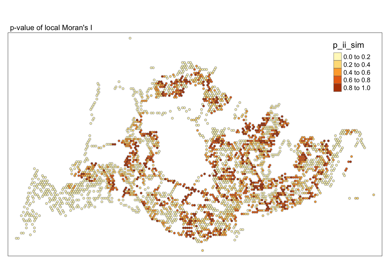
tmap_mode("plot")tmap mode set to plottingmap1 <- tm_shape(lisa) +
tm_fill("ii") +
tm_borders(alpha = 0.5) +
tm_view(set.zoom.limits = c(6,8)) +
tm_layout(main.title = "local Moran's I of Totaltrips",
main.title.size = 0.8)
map2 <- tm_shape(lisa) +
tm_fill("p_ii_sim",
breaks = c(0, 0.001, 0.01, 0.05, 1),
labels = c("0.001", "0.01", "0.05", "Not sig")) +
tm_borders(alpha = 0.5) +
tm_layout(main.title = "p-value of local Moran's I",
main.title.size = 0.8)
tmap_arrange(map1, map2, ncol = 2)Variable(s) "ii" contains positive and negative values, so midpoint is set to 0. Set midpoint = NA to show the full spectrum of the color palette.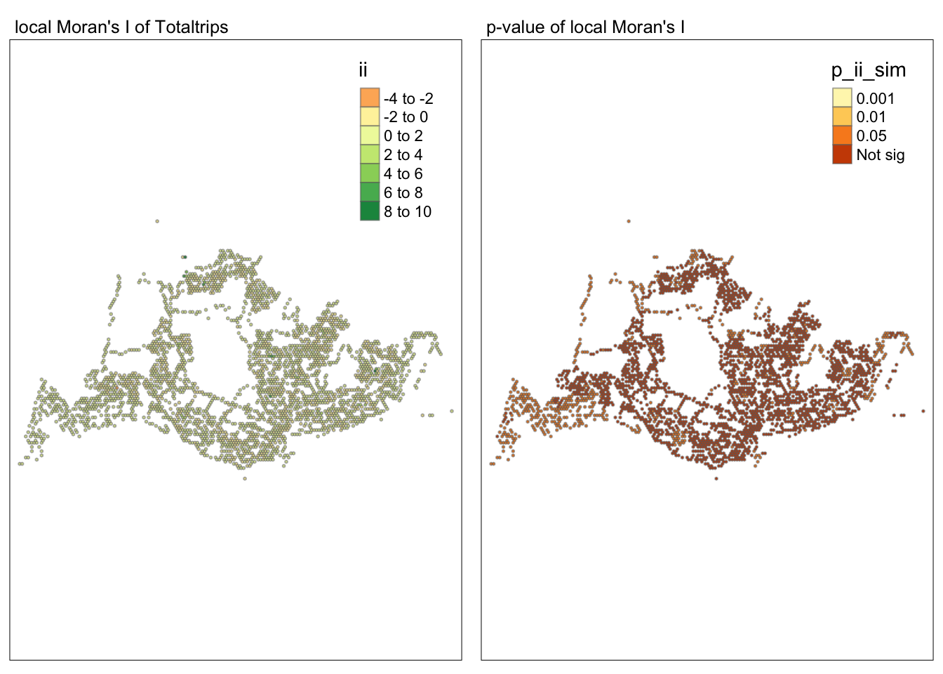
lisa_sig <- lisa  %>%
  filter(p_ii_sim < 0.05)
tmap_mode("plot")
tmap mode set to plottingtm_shape(lisa) +
tm_polygons() +
tm_borders(alpha = 0.5) +
tm_shape(lisa_sig) +
tm_fill("mean") +
tm_borders(alpha = 0.4)Warning: One tm layer group has duplicated layer types, which are omitted. To
draw multiple layers of the same type, use multiple layer groups (i.e. specify
tm_shape prior to each of them).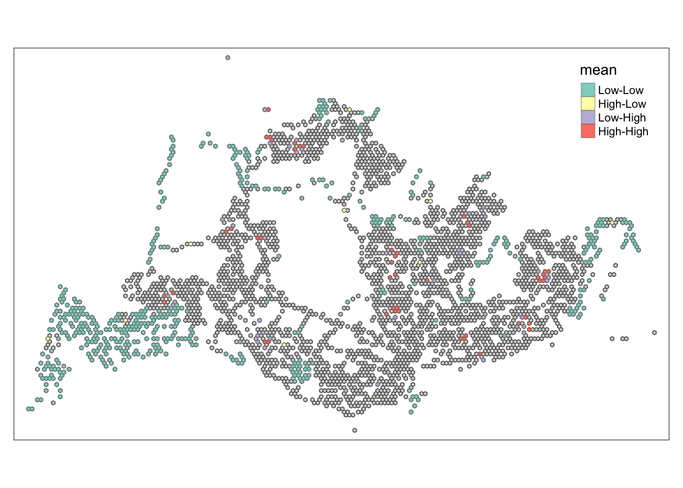
LISA peak time weekend evening
wm_q <- hexagon_count_totaltrips_weekend_evening %>%
  mutate(nb = st_knn(geometry,
                     k=8),
         wt = st_weights(nb),
               .before = 1)
! Polygon provided. Using point on surface.moranI <- global_moran(wm_q$TotalTrips,
wm_q$nb,
wm_q$wt)
glimpse(moranI)List of 2
$ I: num 0.0871
$ K: num 178global_moran_test(wm_q$TotalTrips,
wm_q$nb,
wm_q$wt)
    Moran I test under randomisation

data:  x
weights: listw

Moran I statistic standard deviate = 10.349, p-value < 2.2e-16
alternative hypothesis: greater
sample estimates:
Moran I statistic       Expectation          Variance
8.711577e-02 -3.300330e-04 7.140377e-05 set.seed(1234)global_moran_perm(wm_q$TotalTrips,
wm_q$nb,
wm_q$wt,
nsim = 99)
    Monte-Carlo simulation of Moran I

data:  x
weights: listw
number of simulations + 1: 100

statistic = 0.087116, observed rank = 100, p-value < 2.2e-16
alternative hypothesis: two.sided
lisa <- wm_q %>%
mutate(local_moran = local_moran(
TotalTrips, nb, wt, nsim = 99),
.before = 1) %>%
unnest(local_moran)tmap_mode("plot")tmap mode set to plottingtm_shape(lisa) +
tm_fill("ii") +
tm_borders(alpha = 0.5) +
tm_view(set.zoom.limits = c(6,8)) +
tm_layout(main.title = "local Moran's I of Totaltrips",
main.title.size = 0.8)Variable(s) "ii" contains positive and negative values, so midpoint is set to 0. Set midpoint = NA to show the full spectrum of the color palette.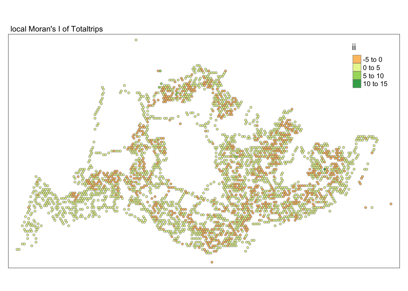
tmap_mode("plot")tmap mode set to plottingtm_shape(lisa) +
tm_fill("p_ii_sim") +
tm_borders(alpha = 0.5) +
tm_layout(main.title = "p-value of local Moran's I",
main.title.size = 0.8)
tmap_mode("plot")tmap mode set to plottingmap1 <- tm_shape(lisa) +
tm_fill("ii") +
tm_borders(alpha = 0.5) +
tm_view(set.zoom.limits = c(6,8)) +
tm_layout(main.title = "local Moran's I of Totaltrips",
main.title.size = 0.8)
map2 <- tm_shape(lisa) +
tm_fill("p_ii_sim",
breaks = c(0, 0.001, 0.01, 0.05, 1),
labels = c("0.001", "0.01", "0.05", "Not sig")) +
tm_borders(alpha = 0.5) +
tm_layout(main.title = "p-value of local Moran's I",
main.title.size = 0.8)
tmap_arrange(map1, map2, ncol = 2)Variable(s) "ii" contains positive and negative values, so midpoint is set to 0. Set midpoint = NA to show the full spectrum of the color palette.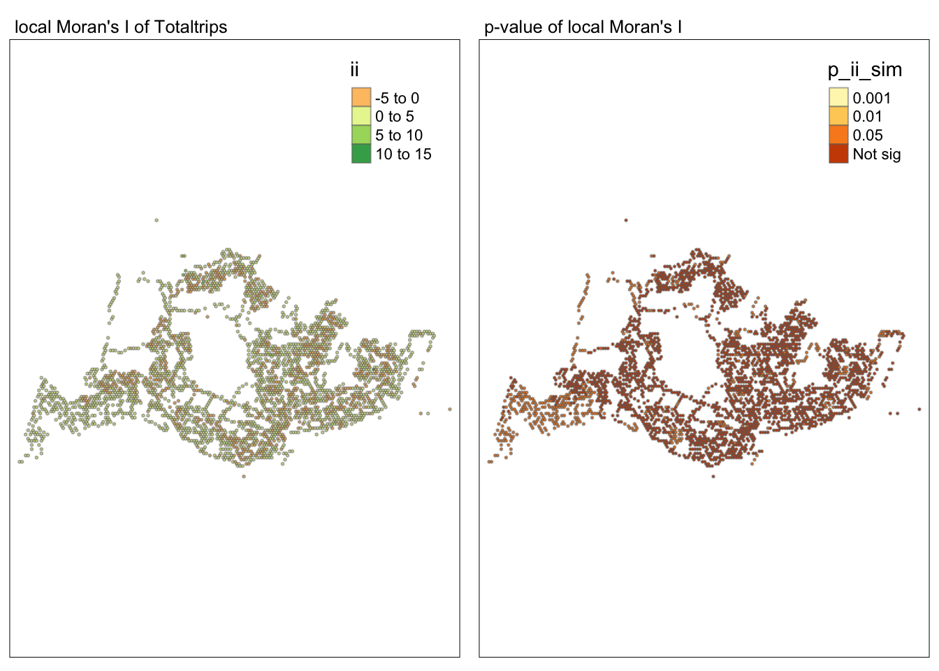
lisa_sig <- lisa  %>%
  filter(p_ii_sim < 0.05)
tmap_mode("plot")
tmap mode set to plottingtm_shape(lisa) +
tm_polygons() +
tm_borders(alpha = 0.5) +
tm_shape(lisa_sig) +
tm_fill("mean") +
tm_borders(alpha = 0.4)Warning: One tm layer group has duplicated layer types, which are omitted. To
draw multiple layers of the same type, use multiple layer groups (i.e. specify
tm_shape prior to each of them).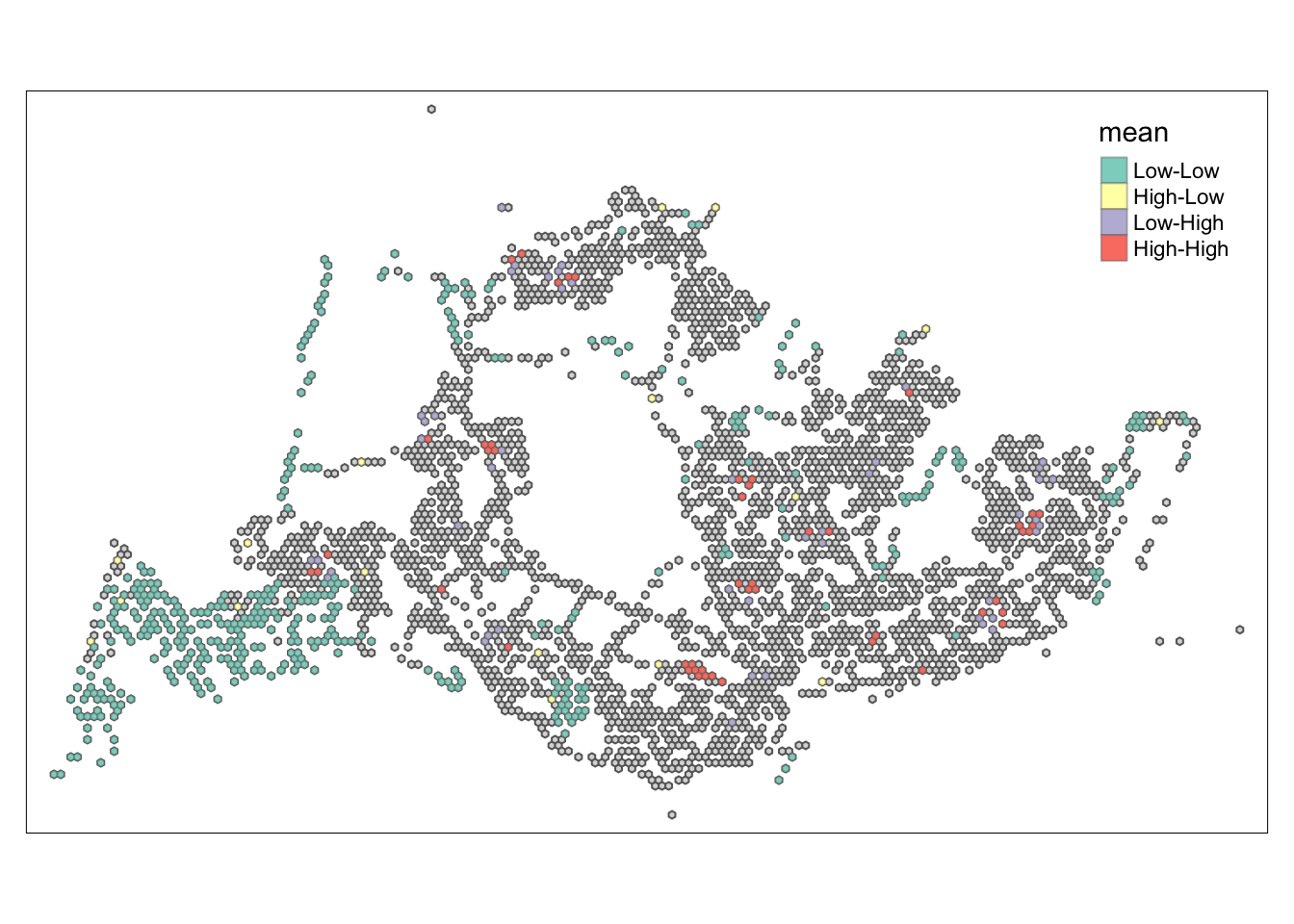
##Conclusion In the complete LISA (Local Indicators of Spatial Association) analysis, we utilize two metrics to identify spatial patterns. Initially, we examine the p-values (displayed in the right-hand map) to determine areas with statistically significant spatial autocorrelation. Regions with p-values less than 0.05 suggest that observed values are unlikely to be randomly distributed and instead exhibit significant spatial correlation with surrounding areas. These significant clusters indicate some form of spatial interaction or mutual influence, potentially due to a combination of geographical, social, economic, or other environmental factors.We need focus on the High-Low and Low-High areas, as these regions are somewhat anomalous compared to others.
Subsequently, we assess the values of the Local Moran’s I (depicted in the left-hand map). Here, positive values denote spatial clusters, indicating similarity in observed values between a region and its neighbors. Negative values reveal spatial outliers, where a region’s values significantly differ from its surroundings, which may highlight unique characteristics or conditions of that area. Further analysis enables us to explore the potential causes behind these clusters and outliers, as well as their specific impacts on the study area.
##Limitation
We have identified regions that may exhibit spatial autocorrelation. Due to the lack of relevant economic and environmental information, further analysis would require us to continue based on the data available.
HCSA
HSCA for weekday morning
wm_idw <- hexagon_count_totaltrips_morning %>%
  mutate(nb = st_contiguity(geometry),
         wts = st_inverse_distance(nb, geometry,
                                   scale = 1,
                                   alpha = 1),
         .before = 1)
! Polygon provided. Using point on surface.HCSA <- wm_idw %>%
mutate(local_Gi = local_gstar_perm(
TotalTrips, nb, wt, nsim = 499),
.before = 1) %>%
unnest(local_Gi)
HCSASimple feature collection with 3047 features and 13 fields
Geometry type: POLYGON
Dimension: XY
Bounding box: xmin: 3720.122 ymin: 26337.76 xmax: 48345.12 ymax: 53040.21
Projected CRS: SVY21 / Singapore TM
# A tibble: 3,047 × 14
gi_star e_gi var_gi p_value p_sim p_folded_sim skewness kurtosis nb
<dbl> <dbl> <dbl> <dbl> <dbl> <dbl> <dbl> <dbl> <nb>
1 -0.744 1.73e-4 7.26e-8 -0.633 0.527 0.128 0.064 3.63 <int>
2 -0.744 1.54e-4 6.00e-8 -0.620 0.535 0.132 0.066 4.33 <int>
3 -0.741 1.58e-4 8.17e-8 -0.539 0.590 0.248 0.124 5.83 <int>
4 -0.527 1.68e-6 0 NaN NaN 1 0.002 NaN <int>
5 -0.741 1.62e-4 7.72e-8 -0.568 0.570 0.112 0.056 4.29 <int>
6 -0.692 1.94e-4 1.50e-7 -0.435 0.663 0.576 0.288 7.55 <int>
7 -0.526 2.78e-6 0 NaN NaN 1 0.002 NaN <int>
8 -0.865 2.12e-4 6.12e-8 -0.782 0.434 0.088 0.044 3.15 <int>
9 -0.525 3.13e-6 0 NaN NaN 1 0.002 NaN <int>
10 -0.716 1.85e-4 1.13e-7 -0.505 0.614 0.244 0.122 5.13 <int>
# ℹ 3,037 more rows
# ℹ 5 more variables: wts <list>, geometry <POLYGON [m]>, grid_id <int>,
# n_colli <int>, TotalTrips <dbl>cbg <- HCSA %>%
ungroup() %>%
select(geometry, TotalTrips, gi_star)ggplot(data = cbg,
aes(x = TotalTrips,
y = gi_star)) +
geom_line() +
theme_light()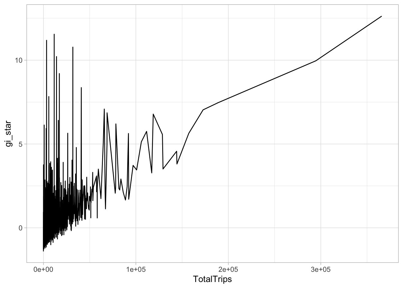
tmap_mode("plot")tmap mode set to plottingtm_shape(HCSA) +
tm_fill("gi_star") +
tm_borders(alpha = 0.5) +
tm_view(set.zoom.limits = c(6,8))Variable(s) "gi_star" contains positive and negative values, so midpoint is set to 0. Set midpoint = NA to show the full spectrum of the color palette.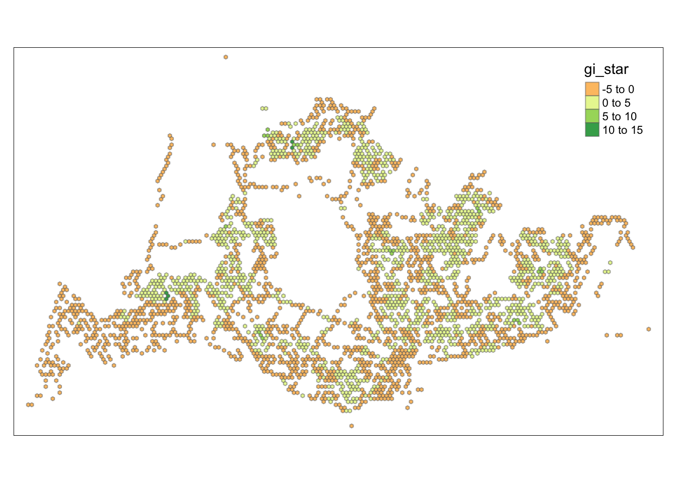
tmap_mode("plot")tmap mode set to plottingtm_shape(HCSA) +
tm_fill("p_sim") +
tm_borders(alpha = 0.5)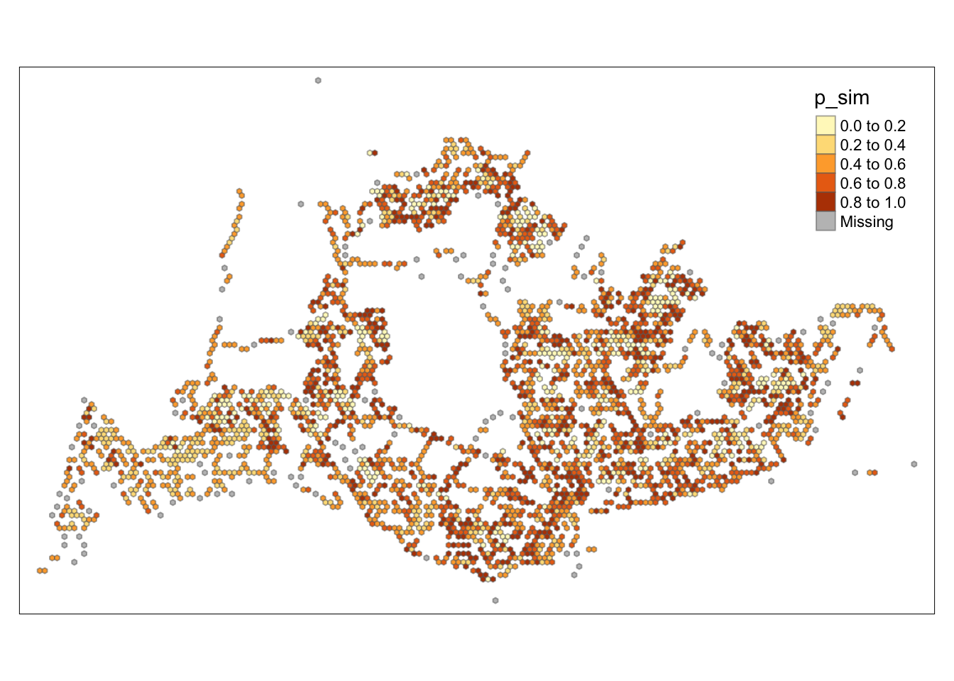
tmap_mode("plot")tmap mode set to plottingmap1 <- tm_shape(HCSA) +
tm_fill("gi_star") +
tm_borders(alpha = 0.5) +
tm_view(set.zoom.limits = c(6,8)) +
tm_layout(main.title = "Gi* of Totaltrips",
main.title.size = 0.8)
map2 <- tm_shape(HCSA) +
tm_fill("p_sim",
breaks = c(0, 0.001, 0.01, 0.05, 1),
labels = c("0.001", "0.01", "0.05", "Not sig")) +
tm_borders(alpha = 0.5) +
tm_layout(main.title = "p-value of Gi*",
main.title.size = 0.8)
tmap_arrange(map1, map2, ncol = 2)Variable(s) "gi_star" contains positive and negative values, so midpoint is set to 0. Set midpoint = NA to show the full spectrum of the color palette.
HCSA_sig <- HCSA  %>%
  filter(p_sim < 0.05)
tmap_mode("plot")
tmap mode set to plottingtm_shape(HCSA) +
tm_polygons() +
tm_borders(alpha = 0.5) +
tm_shape(HCSA_sig) +
tm_fill("gi_star") +
tm_borders(alpha = 0.4)Warning: One tm layer group has duplicated layer types, which are omitted. To
draw multiple layers of the same type, use multiple layer groups (i.e. specify
tm_shape prior to each of them).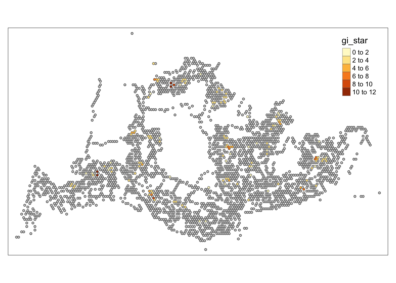
HCSA for weekday afternoon
wm_idw <- hexagon_count_totaltrips_afternoon %>%
  mutate(nb = st_contiguity(geometry),
         wts = st_inverse_distance(nb, geometry,
                                   scale = 1,
                                   alpha = 1),
         .before = 1)
! Polygon provided. Using point on surface.HCSA <- wm_idw %>%
mutate(local_Gi = local_gstar_perm(
TotalTrips, nb, wt, nsim = 499),
.before = 1) %>%
unnest(local_Gi)
HCSASimple feature collection with 3054 features and 12 fields
Geometry type: POLYGON
Dimension: XY
Bounding box: xmin: 3720.122 ymin: 26337.76 xmax: 48345.12 ymax: 53040.21
Projected CRS: SVY21 / Singapore TM
# A tibble: 3,054 × 13
gi_star e_gi var_gi p_value p_sim p_folded_sim skewness kurtosis nb
<dbl> <dbl> <dbl> <dbl> <dbl> <dbl> <dbl> <dbl> <nb>
1 -0.501 1.87e-4 2.85e-7 -0.320 0.749 0.212 0.106 11.0 <int>
2 -0.501 1.52e-4 9.22e-8 -0.446 0.656 0.236 0.118 7.08 <int>
3 -0.466 1.64e-4 1.10e-7 -0.379 0.705 0.648 0.324 5.68 <int>
4 -0.361 9.83e-6 0 NaN NaN 1 0.002 NaN <int>
5 -0.466 1.84e-4 2.00e-7 -0.327 0.743 0.088 0.044 11.9 <int>
6 -0.426 1.35e-4 4.79e-8 -0.329 0.743 0.904 0.452 5.08 <int>
7 -0.363 8.68e-6 0 NaN NaN 1 0.002 NaN <int>
8 -0.550 2.71e-4 2.20e-7 -0.475 0.635 0.052 0.026 8.24 <int>
9 -0.358 1.28e-5 0 NaN NaN 1 0.002 NaN <int>
10 -0.443 2.04e-4 1.12e-7 -0.456 0.648 0.172 0.086 6.62 <int>
# ℹ 3,044 more rows
# ℹ 4 more variables: wts <list>, geometry <POLYGON [m]>, grid_id <int>,
# TotalTrips <dbl>cbg <- HCSA %>%
ungroup() %>%
select(geometry, TotalTrips, gi_star)ggplot(data = cbg,
aes(x = TotalTrips,
y = gi_star)) +
geom_line() +
theme_light()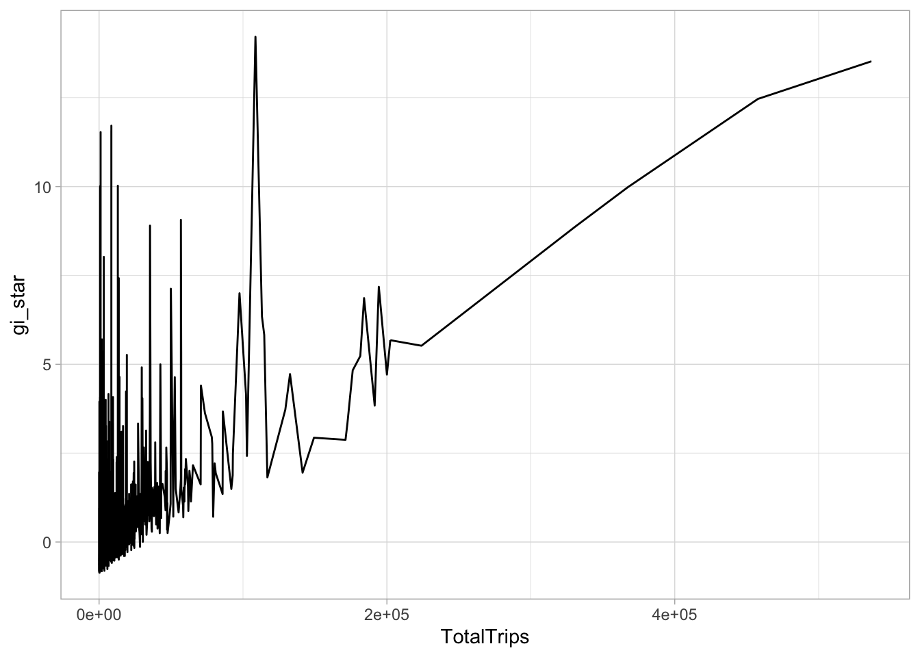
tmap_mode("plot")tmap mode set to plottingtm_shape(HCSA) +
tm_fill("gi_star") +
tm_borders(alpha = 0.5) +
tm_view(set.zoom.limits = c(6,8))Variable(s) "gi_star" contains positive and negative values, so midpoint is set to 0. Set midpoint = NA to show the full spectrum of the color palette.
tmap_mode("plot")tmap mode set to plottingtm_shape(HCSA) +
tm_fill("p_sim") +
tm_borders(alpha = 0.5)
tmap_mode("plot")tmap mode set to plottingmap1 <- tm_shape(HCSA) +
tm_fill("gi_star") +
tm_borders(alpha = 0.5) +
tm_view(set.zoom.limits = c(6,8)) +
tm_layout(main.title = "Gi* of Totaltrips",
main.title.size = 0.8)
map2 <- tm_shape(HCSA) +
tm_fill("p_sim",
breaks = c(0, 0.001, 0.01, 0.05, 1),
labels = c("0.001", "0.01", "0.05", "Not sig")) +
tm_borders(alpha = 0.5) +
tm_layout(main.title = "p-value of Gi*",
main.title.size = 0.8)
tmap_arrange(map1, map2, ncol = 2)Variable(s) "gi_star" contains positive and negative values, so midpoint is set to 0. Set midpoint = NA to show the full spectrum of the color palette.
HCSA_sig <- HCSA  %>%
  filter(p_sim < 0.05)
tmap_mode("plot")
tmap mode set to plottingtm_shape(HCSA) +
tm_polygons() +
tm_borders(alpha = 0.5) +
tm_shape(HCSA_sig) +
tm_fill("gi_star") +
tm_borders(alpha = 0.4)Warning: One tm layer group has duplicated layer types, which are omitted. To
draw multiple layers of the same type, use multiple layer groups (i.e. specify
tm_shape prior to each of them).
HCSA for weekday afternoon
wm_idw <- hexagon_count_totaltrips_afternoon %>%
  mutate(nb = st_contiguity(geometry),
         wts = st_inverse_distance(nb, geometry,
                                   scale = 1,
                                   alpha = 1),
         .before = 1)
! Polygon provided. Using point on surface.HCSA <- wm_idw %>%
mutate(local_Gi = local_gstar_perm(
TotalTrips, nb, wt, nsim = 499),
.before = 1) %>%
unnest(local_Gi)
HCSASimple feature collection with 3054 features and 12 fields
Geometry type: POLYGON
Dimension: XY
Bounding box: xmin: 3720.122 ymin: 26337.76 xmax: 48345.12 ymax: 53040.21
Projected CRS: SVY21 / Singapore TM
# A tibble: 3,054 × 13
gi_star e_gi var_gi p_value p_sim p_folded_sim skewness kurtosis nb
<dbl> <dbl> <dbl> <dbl> <dbl> <dbl> <dbl> <dbl> <nb>
1 -0.501 2.30e-4 3.22e-7 -0.377 0.706 0.256 0.128 6.88 <int>
2 -0.501 1.73e-4 1.10e-7 -0.471 0.638 0.188 0.094 6.43 <int>
3 -0.466 1.71e-4 1.07e-7 -0.408 0.684 0.6 0.3 5.85 <int>
4 -0.361 9.83e-6 0 NaN NaN 1 0.002 NaN <int>
5 -0.466 1.93e-4 2.30e-7 -0.324 0.746 0.096 0.048 13.8 <int>
6 -0.426 1.44e-4 6.84e-8 -0.311 0.756 0.884 0.442 7.75 <int>
7 -0.363 8.68e-6 0 NaN NaN 1 0.002 NaN <int>
8 -0.550 2.59e-4 1.07e-7 -0.643 0.520 0.044 0.022 4.41 <int>
9 -0.358 1.28e-5 0 NaN NaN 1 0.002 NaN <int>
10 -0.443 2.11e-4 1.47e-7 -0.415 0.678 0.192 0.096 7.04 <int>
# ℹ 3,044 more rows
# ℹ 4 more variables: wts <list>, geometry <POLYGON [m]>, grid_id <int>,
# TotalTrips <dbl>cbg <- HCSA %>%
ungroup() %>%
select(geometry, TotalTrips, gi_star)ggplot(data = cbg,
aes(x = TotalTrips,
y = gi_star)) +
geom_line() +
theme_light()
tmap_mode("plot")tmap mode set to plottingtm_shape(HCSA) +
tm_fill("gi_star") +
tm_borders(alpha = 0.5) +
tm_view(set.zoom.limits = c(6,8))Variable(s) "gi_star" contains positive and negative values, so midpoint is set to 0. Set midpoint = NA to show the full spectrum of the color palette.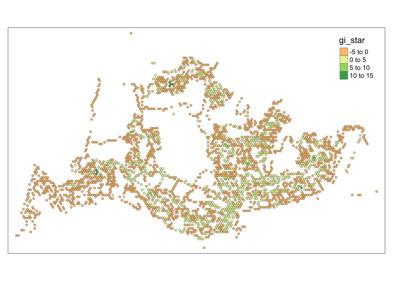
tmap_mode("plot")tmap mode set to plottingtm_shape(HCSA) +
tm_fill("p_sim") +
tm_borders(alpha = 0.5)
tmap_mode("plot")tmap mode set to plottingmap1 <- tm_shape(HCSA) +
tm_fill("gi_star") +
tm_borders(alpha = 0.5) +
tm_view(set.zoom.limits = c(6,8)) +
tm_layout(main.title = "Gi* of Totaltrips",
main.title.size = 0.8)
map2 <- tm_shape(HCSA) +
tm_fill("p_sim",
breaks = c(0, 0.001, 0.01, 0.05, 1),
labels = c("0.001", "0.01", "0.05", "Not sig")) +
tm_borders(alpha = 0.5) +
tm_layout(main.title = "p-value of Gi*",
main.title.size = 0.8)
tmap_arrange(map1, map2, ncol = 2)Variable(s) "gi_star" contains positive and negative values, so midpoint is set to 0. Set midpoint = NA to show the full spectrum of the color palette.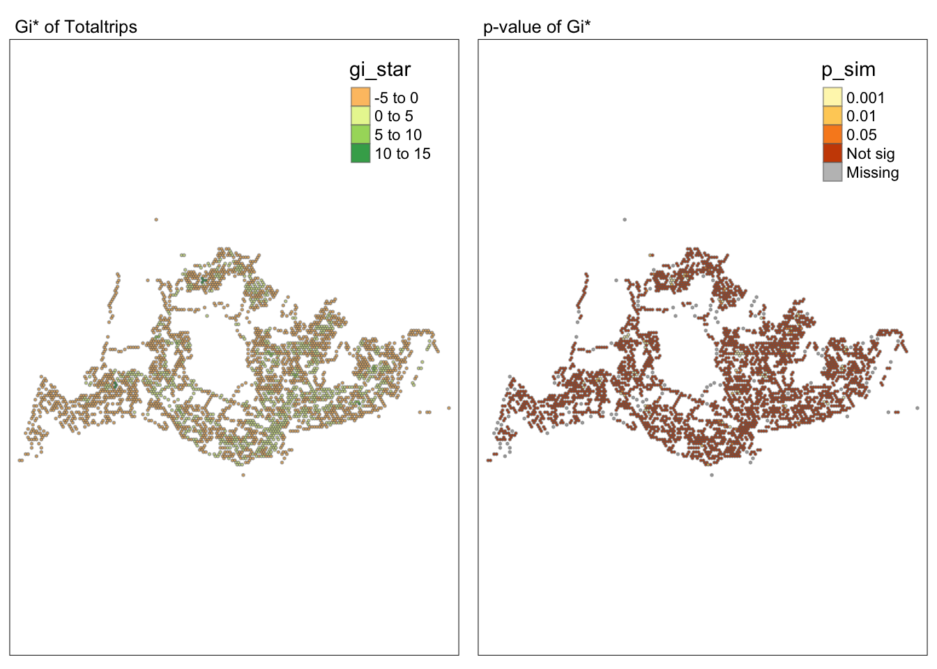
HCSA_sig <- HCSA  %>%
  filter(p_sim < 0.05)
tmap_mode("plot")
tmap mode set to plottingtm_shape(HCSA) +
tm_polygons() +
tm_borders(alpha = 0.5) +
tm_shape(HCSA_sig) +
tm_fill("gi_star") +
tm_borders(alpha = 0.4)Warning: One tm layer group has duplicated layer types, which are omitted. To
draw multiple layers of the same type, use multiple layer groups (i.e. specify
tm_shape prior to each of them).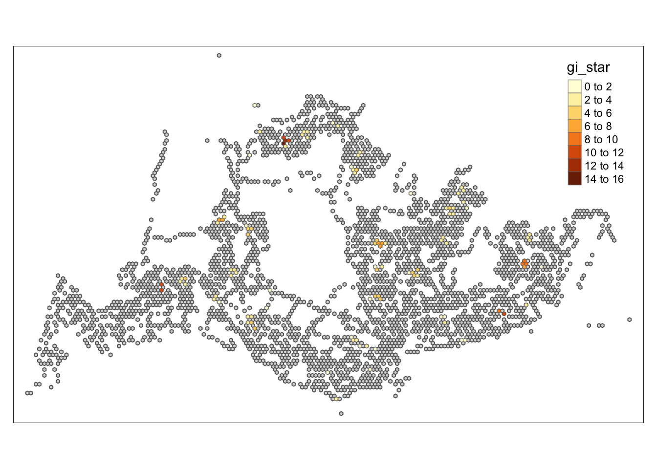
HCSA for weekend morning
wm_idw <- hexagon_count_totaltrips_weekend_morning %>%
  mutate(nb = st_contiguity(geometry),
         wts = st_inverse_distance(nb, geometry,
                                   scale = 1,
                                   alpha = 1),
         .before = 1)
! Polygon provided. Using point on surface.HCSA <- wm_idw %>%
mutate(local_Gi = local_gstar_perm(
TotalTrips, nb, wt, nsim = 499),
.before = 1) %>%
unnest(local_Gi)
HCSASimple feature collection with 3050 features and 12 fields
Geometry type: POLYGON
Dimension: XY
Bounding box: xmin: 3720.122 ymin: 26337.76 xmax: 48345.12 ymax: 53040.21
Projected CRS: SVY21 / Singapore TM
# A tibble: 3,050 × 13
gi_star e_gi var_gi p_value p_sim p_folded_sim skewness kurtosis nb
<dbl> <dbl> <dbl> <dbl> <dbl> <dbl> <dbl> <dbl> <nb>
1 -0.669 1.62e-4 8.76e-8 -0.547 0.585 0.016 0.008 4.61 <int>
2 -0.669 1.95e-4 2.18e-7 -0.416 0.677 0.016 0.008 7.70 <int>
3 -0.647 1.86e-4 3.42e-7 -0.299 0.765 0.368 0.184 8.98 <int>
4 -0.468 3.54e-6 0 NaN NaN 1 0.002 NaN <int>
5 -0.647 1.66e-4 8.82e-8 -0.521 0.603 0.096 0.048 9.19 <int>
6 -0.596 1.69e-4 7.97e-8 -0.471 0.638 0.6 0.3 4.56 <int>
7 -0.459 9.83e-6 0 NaN NaN 1 0.002 NaN <int>
8 -0.754 2.39e-4 1.05e-7 -0.658 0.511 0.048 0.024 6.72 <int>
9 -0.465 5.64e-6 0 NaN NaN 1 0.002 NaN <int>
10 -0.595 1.83e-4 5.62e-8 -0.617 0.537 0.208 0.102 3.93 <int>
# ℹ 3,040 more rows
# ℹ 4 more variables: wts <list>, geometry <POLYGON [m]>, grid_id <int>,
# TotalTrips <dbl>cbg <- HCSA %>%
ungroup() %>%
select(geometry, TotalTrips, gi_star)ggplot(data = cbg,
aes(x = TotalTrips,
y = gi_star)) +
geom_line() +
theme_light()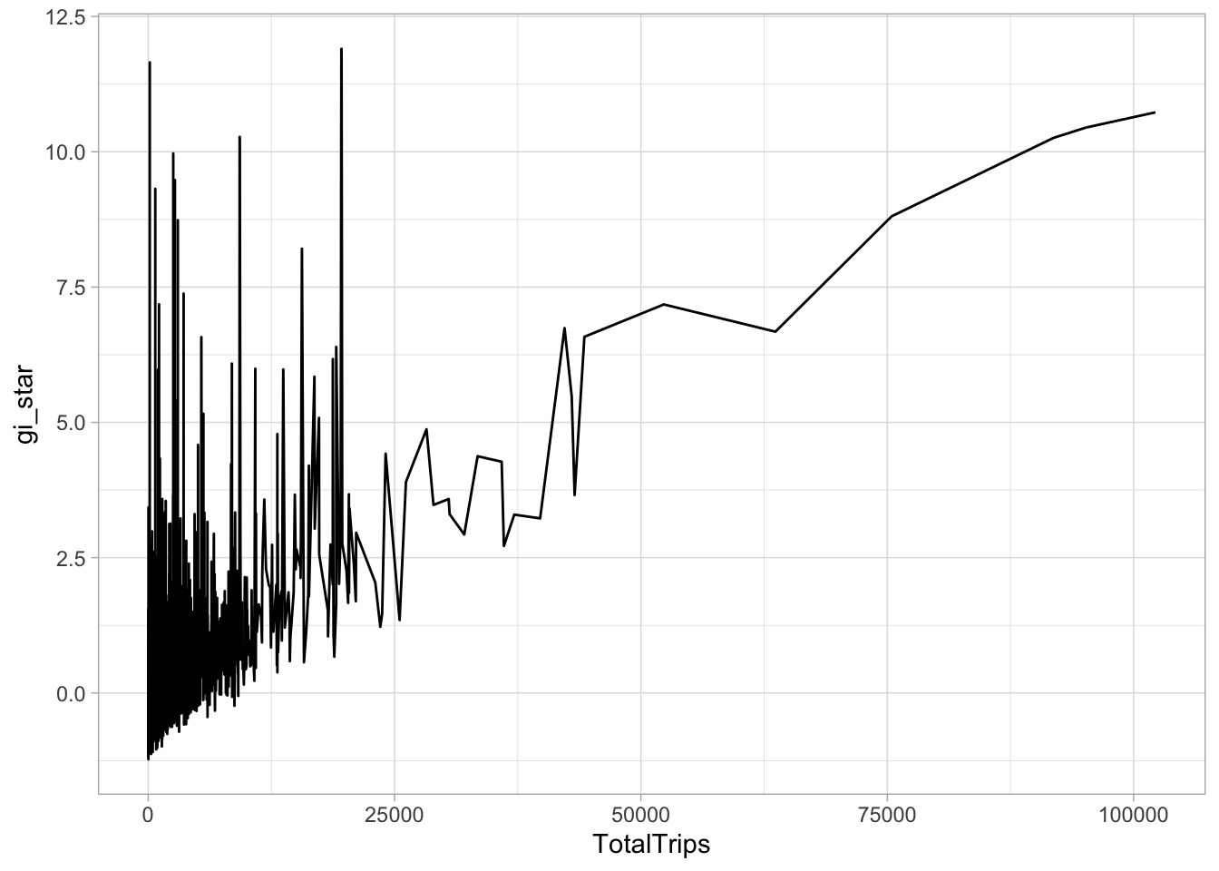
tmap_mode("plot")tmap mode set to plottingtm_shape(HCSA) +
tm_fill("gi_star") +
tm_borders(alpha = 0.5) +
tm_view(set.zoom.limits = c(6,8))Variable(s) "gi_star" contains positive and negative values, so midpoint is set to 0. Set midpoint = NA to show the full spectrum of the color palette.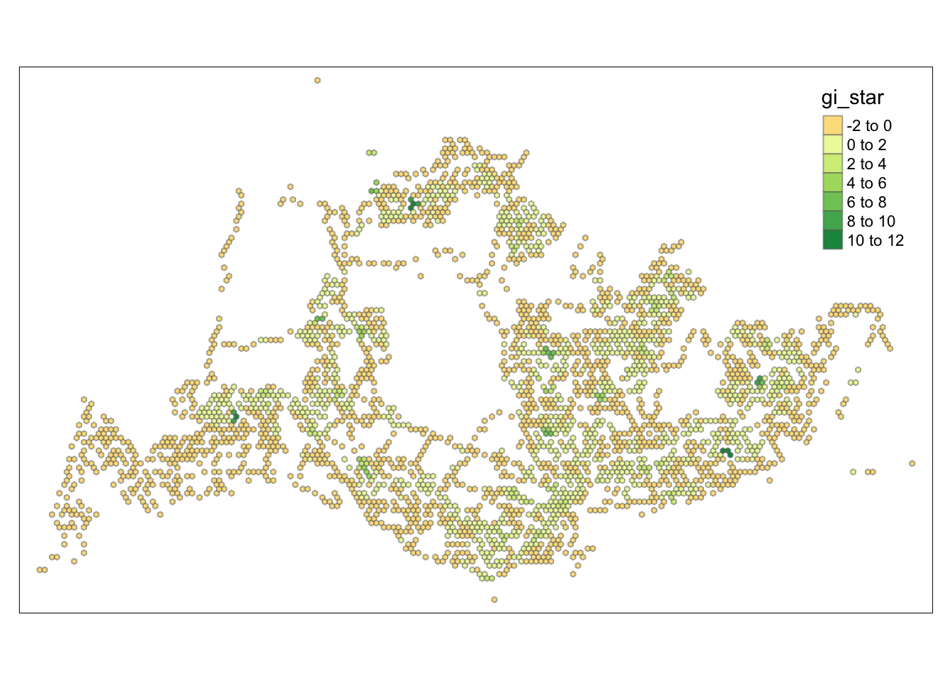
tmap_mode("plot")tmap mode set to plottingtm_shape(HCSA) +
tm_fill("p_sim") +
tm_borders(alpha = 0.5)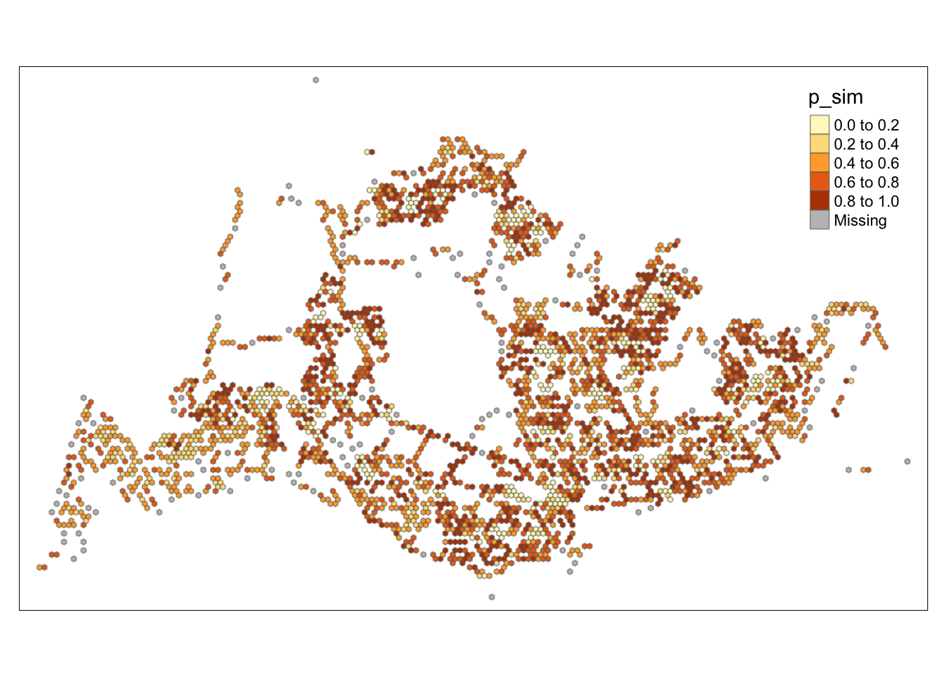
tmap_mode("plot")tmap mode set to plottingmap1 <- tm_shape(HCSA) +
tm_fill("gi_star") +
tm_borders(alpha = 0.5) +
tm_view(set.zoom.limits = c(6,8)) +
tm_layout(main.title = "Gi* of Totaltrips",
main.title.size = 0.8)
map2 <- tm_shape(HCSA) +
tm_fill("p_sim",
breaks = c(0, 0.001, 0.01, 0.05, 1),
labels = c("0.001", "0.01", "0.05", "Not sig")) +
tm_borders(alpha = 0.5) +
tm_layout(main.title = "p-value of Gi*",
main.title.size = 0.8)
tmap_arrange(map1, map2, ncol = 2)Variable(s) "gi_star" contains positive and negative values, so midpoint is set to 0. Set midpoint = NA to show the full spectrum of the color palette.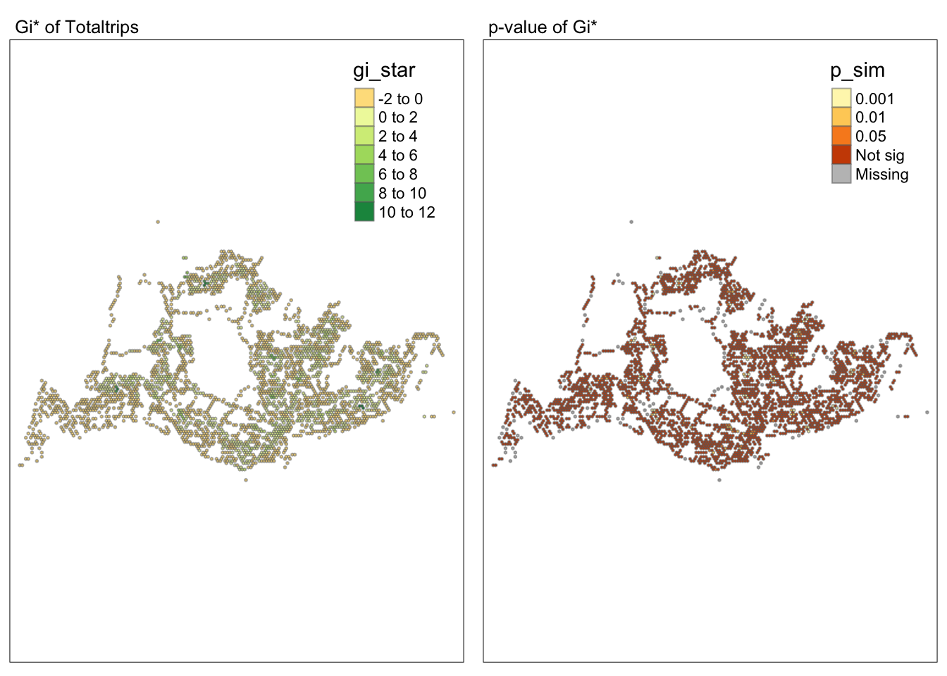
HCSA_sig <- HCSA  %>%
  filter(p_sim < 0.05)
tmap_mode("plot")
tmap mode set to plottingtm_shape(HCSA) +
tm_polygons() +
tm_borders(alpha = 0.5) +
tm_shape(HCSA_sig) +
tm_fill("gi_star") +
tm_borders(alpha = 0.4)Warning: One tm layer group has duplicated layer types, which are omitted. To
draw multiple layers of the same type, use multiple layer groups (i.e. specify
tm_shape prior to each of them).
HCSA for weekend evening
wm_idw <- hexagon_count_totaltrips_weekend_evening %>%
  mutate(nb = st_contiguity(geometry),
         wts = st_inverse_distance(nb, geometry,
                                   scale = 1,
                                   alpha = 1),
         .before = 1)
! Polygon provided. Using point on surface.HCSA <- wm_idw %>%
mutate(local_Gi = local_gstar_perm(
TotalTrips, nb, wt, nsim = 499),
.before = 1) %>%
unnest(local_Gi)
HCSASimple feature collection with 3031 features and 12 fields
Geometry type: POLYGON
Dimension: XY
Bounding box: xmin: 3720.122 ymin: 26337.76 xmax: 48345.12 ymax: 53040.21
Projected CRS: SVY21 / Singapore TM
# A tibble: 3,031 × 13
gi_star e_gi var_gi p_value p_sim p_folded_sim skewness kurtosis nb
<dbl> <dbl> <dbl> <dbl> <dbl> <dbl> <dbl> <dbl> <nb>
1 -0.545 1.53e-4 1.05e-7 -0.447 0.655 0.132 0.066 6.26 <int>
2 -0.545 2.10e-4 4.21e-7 -0.310 0.757 0.196 0.098 9.42 <int>
3 -0.522 1.72e-4 2.08e-7 -0.329 0.742 0.54 0.27 8.64 <int>
4 -0.387 7.11e-6 0 NaN NaN 1 0.002 NaN <int>
5 -0.522 2.12e-4 2.78e-7 -0.361 0.718 0.064 0.032 11.8 <int>
6 -0.472 1.86e-4 1.49e-7 -0.350 0.726 0.76 0.38 5.41 <int>
7 -0.390 4.61e-6 0 NaN NaN 1 0.002 NaN <int>
8 -0.607 2.55e-4 2.26e-7 -0.457 0.648 0.044 0.022 9.36 <int>
9 -0.388 6.45e-6 0 NaN NaN 1 0.002 NaN <int>
10 -0.450 2.28e-4 2.19e-7 -0.350 0.726 0.48 0.24 10.4 <int>
# ℹ 3,021 more rows
# ℹ 4 more variables: wts <list>, geometry <POLYGON [m]>, grid_id <int>,
# TotalTrips <dbl>cbg <- HCSA %>%
ungroup() %>%
select(geometry, TotalTrips, gi_star)ggplot(data = cbg,
aes(x = TotalTrips,
y = gi_star)) +
geom_line() +
theme_light()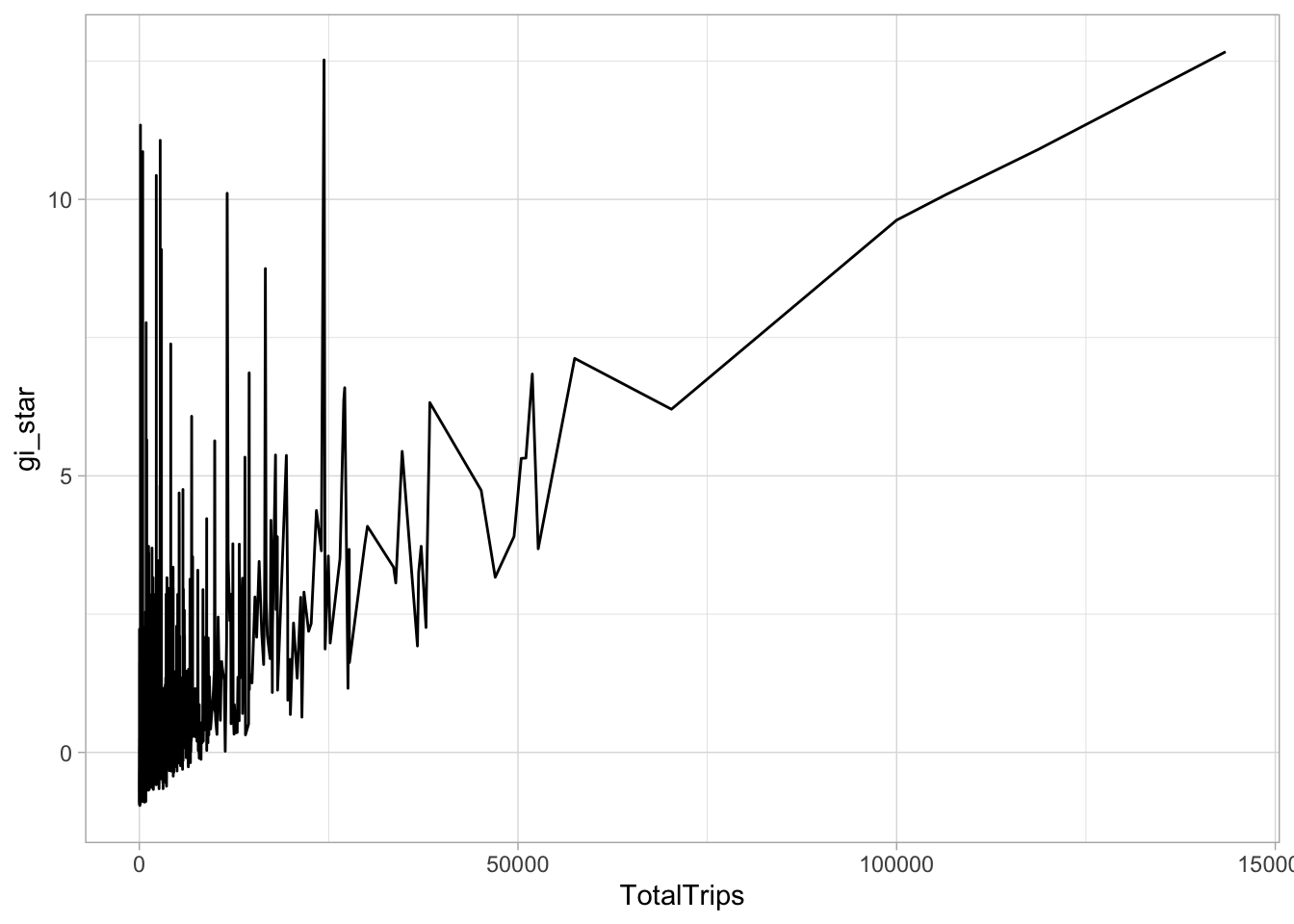
tmap_mode("plot")tmap mode set to plottingtm_shape(HCSA) +
tm_fill("gi_star") +
tm_borders(alpha = 0.5) +
tm_view(set.zoom.limits = c(6,8))Variable(s) "gi_star" contains positive and negative values, so midpoint is set to 0. Set midpoint = NA to show the full spectrum of the color palette.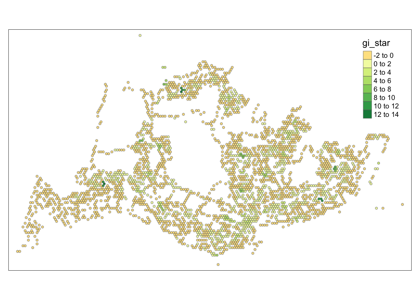
tmap_mode("plot")tmap mode set to plottingtm_shape(HCSA) +
tm_fill("p_sim") +
tm_borders(alpha = 0.5)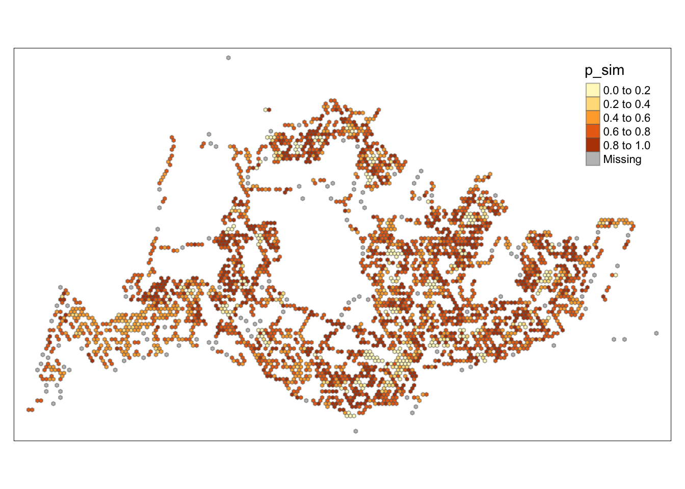
tmap_mode("plot")tmap mode set to plottingmap1 <- tm_shape(HCSA) +
tm_fill("gi_star") +
tm_borders(alpha = 0.5) +
tm_view(set.zoom.limits = c(6,8)) +
tm_layout(main.title = "Gi* of Totaltrips",
main.title.size = 0.8)
map2 <- tm_shape(HCSA) +
tm_fill("p_sim",
breaks = c(0, 0.001, 0.01, 0.05, 1),
labels = c("0.001", "0.01", "0.05", "Not sig")) +
tm_borders(alpha = 0.5) +
tm_layout(main.title = "p-value of Gi*",
main.title.size = 0.8)
tmap_arrange(map1, map2, ncol = 2)Variable(s) "gi_star" contains positive and negative values, so midpoint is set to 0. Set midpoint = NA to show the full spectrum of the color palette.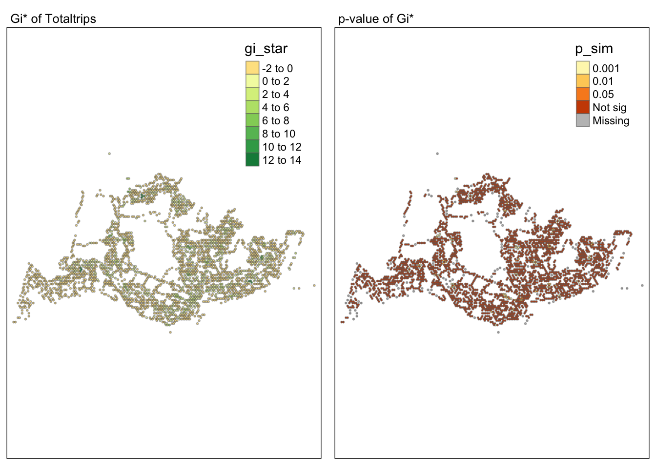
HCSA_sig <- HCSA  %>%
  filter(p_sim < 0.05)
tmap_mode("plot")
tmap mode set to plottingtm_shape(HCSA) +
tm_polygons() +
tm_borders(alpha = 0.5) +
tm_shape(HCSA_sig) +
tm_fill("gi_star") +
tm_borders(alpha = 0.4)Warning: One tm layer group has duplicated layer types, which are omitted. To
draw multiple layers of the same type, use multiple layer groups (i.e. specify
tm_shape prior to each of them).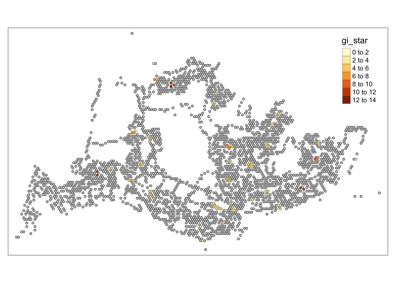
Conclusion
Through the hot and cold spot analysis, there are four areas with notably high GI values that we can focus on in subsequent analyses. Due to the lack of relevant economic and environmental information, we can only determine that these four areas significantly exceed the average level. Moving forward, we can delve into the reasons behind this by gathering more data and documentation.